R: Binomial sampling with a general continuous prior
binogcp
R Documentation
Binomial sampling with a general continuous prior
Description
Evaluates and plots the posterior density for pi, the probability
of a success in a Bernoulli trial, with binomial sampling and a general
continuous prior on pi
Usage
binogcp(x, n, density = c("uniform", "beta", "exp", "normal", "user"),
  params = c(0, 1), n.pi = 1000, pi = NULL, pi.prior = NULL,
  plot = TRUE)
Arguments
x
the number of observed successes in the binomial experiment.
n
the number of trials in the binomial experiment.
density
may be one of "beta", "exp", "normal", "student", "uniform"
or "user"
params
if density is one of the parameteric forms then then a vector
of parameters must be supplied. beta: a, b exp: rate normal: mean, sd
uniform: min, max
n.pi
the number of possible pi values in the prior
pi
a vector of possibilities for the probability of success in a
single trial. This must be set if density = "user".
pi.prior
the associated prior probability mass. This must be set if
density = "user".
plot
if TRUE then a plot showing the prior and the posterior
will be produced.
Value
A list will be returned with the following components:
likelihood
the scaled likelihood function for pi given
x and n
posterior
the posterior probability of
pi given x and n
pi
the vector of possible
pi values used in the prior
pi.prior
the associated
probability mass for the values in pi
See Also
binobpbinodp
Examples
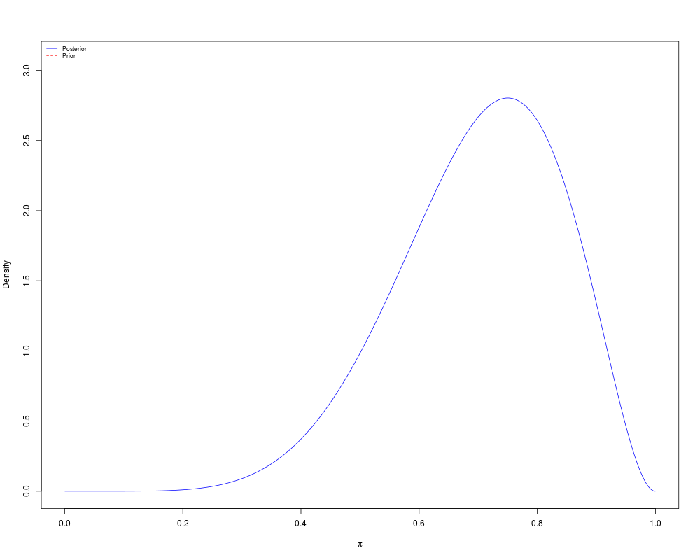
## simplest call with 6 successes observed in 8 trials and a continuous
## uniform prior
binogcp(6, 8)
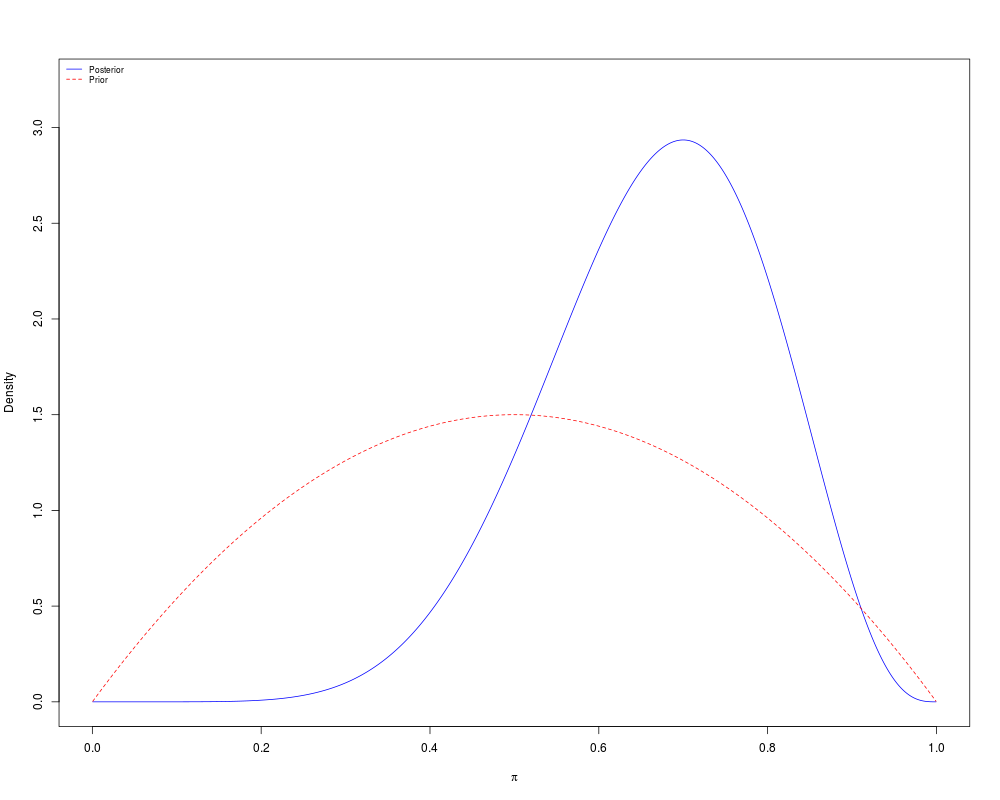
## 6 successes, 8 trials and a Beta(2, 2) prior
binogcp(6, 8,density = "beta", params = c(2, 2))
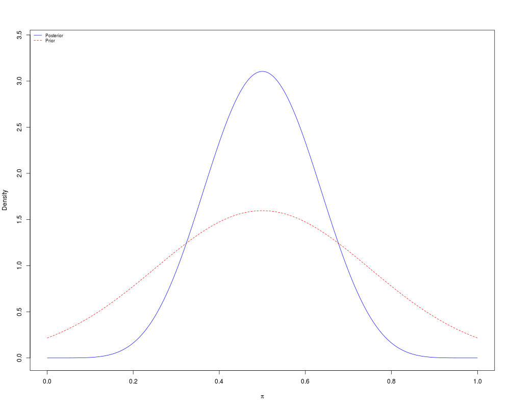
## 5 successes, 10 trials and a N(0.5, 0.25) prior
binogcp(5, 10, density = "normal", params = c(0.5, 0.25))
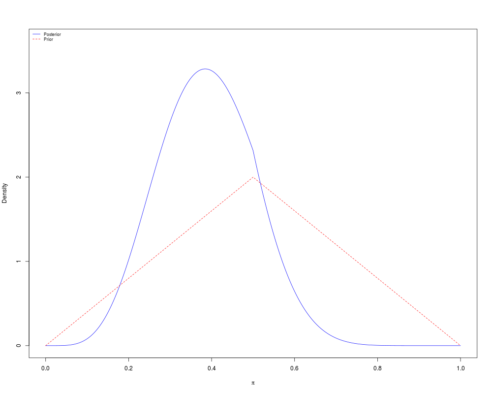
## 4 successes, 12 trials with a user specified triangular continuous prior
pi = seq(0, 1,by = 0.001)
pi.prior = rep(0, length(pi))
priorFun = createPrior(x = c(0, 0.5, 1), wt = c(0, 2, 0))
pi.prior = priorFun(pi)
results = binogcp(4, 12, "user", pi = pi, pi.prior = pi.prior)
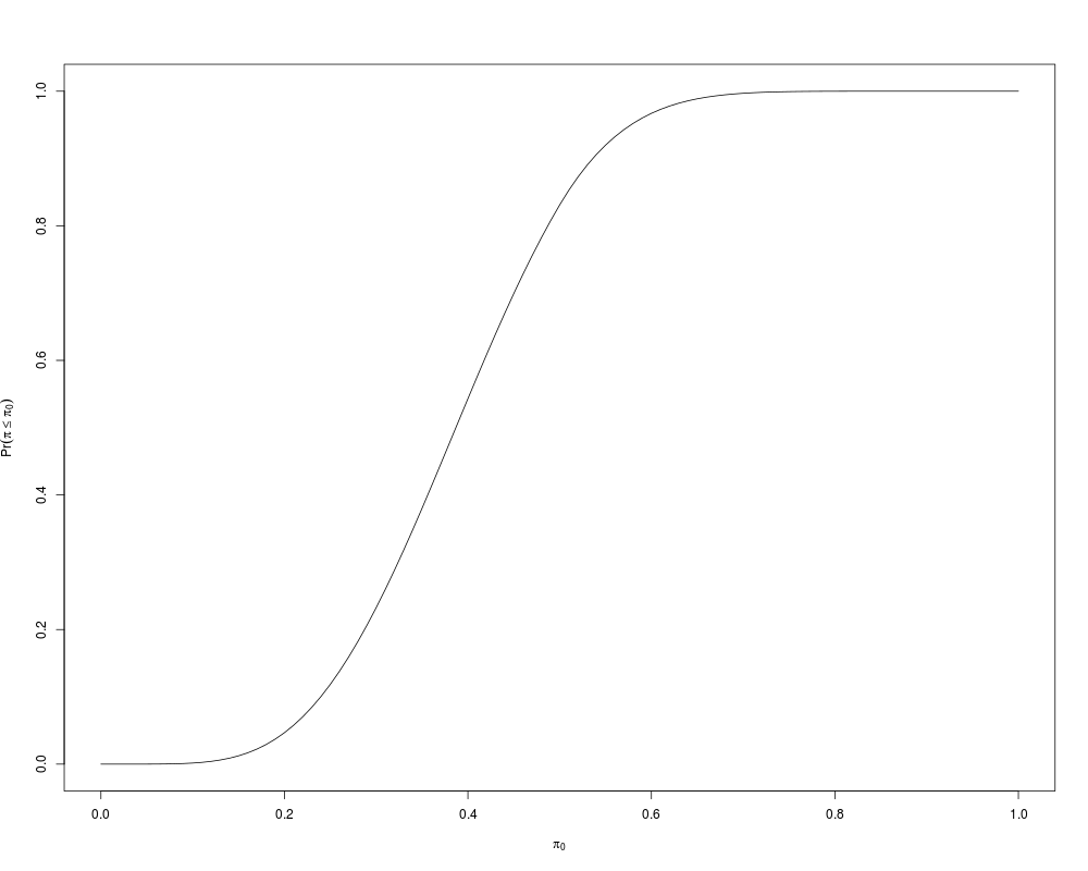
## find the posterior CDF using the previous example and Simpson's rule
myCdf = cdf(results)
plot(myCdf, type = "l", xlab = expression(pi[0]),
ylab = expression(Pr(pi <= pi[0])))
## use the quantile function to find the 95% credible region.
qtls = quantile(results, probs = c(0.025, 0.975))
cat(paste("Approximate 95% credible interval : ["
, round(qtls[1], 4), " ", round(qtls, 4), "]\n", sep = ""))
## find the posterior mean, variance and std. deviation
## using the output from the previous example
post.mean = mean(results)
post.var = var(results)
post.sd = sd(results)
# calculate an approximate 95% credible region using the posterior mean and
# std. deviation
lb = post.mean - qnorm(0.975) * post.sd
ub = post.mean + qnorm(0.975) * post.sd
cat(paste("Approximate 95% credible interval : ["
, round(lb, 4), " ", round(ub, 4), "]\n", sep = ""))
Results
R version 3.3.1 (2016-06-21) -- "Bug in Your Hair"
Copyright (C) 2016 The R Foundation for Statistical Computing
Platform: x86_64-pc-linux-gnu (64-bit)

R is free software and comes with ABSOLUTELY NO WARRANTY.
You are welcome to redistribute it under certain conditions.
Type 'license()' or 'licence()' for distribution details.

R is a collaborative project with many contributors.
Type 'contributors()' for more information and
'citation()' on how to cite R or R packages in publications.

Type 'demo()' for some demos, 'help()' for on-line help, or
'help.start()' for an HTML browser interface to help.
Type 'q()' to quit R.

> library(Bolstad)

Attaching package: 'Bolstad'

The following objects are masked from 'package:stats':

    IQR, sd, var

> png(filename="/home/ddbj/snapshot/RGM3/R_CC/result/Bolstad/binogcp.Rd_%03d_medium.png", width=480, height=480)
> ### Name: binogcp
> ### Title: Binomial sampling with a general continuous prior
> ### Aliases: binogcp
> ### Keywords: misc
>
> ### ** Examples
>
>
> ## simplest call with 6 successes observed in 8 trials and a continuous
> ## uniform prior
> binogcp(6, 8)
>
> ## 6 successes, 8 trials and a Beta(2, 2) prior
> binogcp(6, 8,density = "beta", params = c(2, 2))
>
> ## 5 successes, 10 trials and a N(0.5, 0.25) prior
> binogcp(5, 10, density = "normal", params = c(0.5, 0.25))
>
> ## 4 successes, 12 trials with a user specified triangular continuous prior
> pi = seq(0, 1,by = 0.001)
> pi.prior = rep(0, length(pi))
> priorFun = createPrior(x = c(0, 0.5, 1), wt = c(0, 2, 0))
> pi.prior = priorFun(pi)
> results = binogcp(4, 12, "user", pi = pi, pi.prior = pi.prior)
>
> ## find the posterior CDF using the previous example and Simpson's rule
> myCdf = cdf(results)
> plot(myCdf, type = "l", xlab = expression(pi[0]),
+ 	   ylab = expression(Pr(pi <= pi[0])))
>
> ## use the quantile function to find the 95% credible region.
> qtls = quantile(results, probs = c(0.025, 0.975))
> cat(paste("Approximate 95% credible interval : ["
+ 	, round(qtls[1], 4), " ", round(qtls, 4), "]\n", sep = ""))
Approximate 95% credible interval : [0.1741 0.1741]
 Approximate 95% credible interval : [0.1741 0.6137]
>
> ## find the posterior mean, variance and std. deviation
> ## using the output from the previous example
> post.mean = mean(results)
> post.var = var(results)
> post.sd = sd(results)
>
> # calculate an approximate 95% credible region using the posterior mean and
> # std. deviation
> lb = post.mean - qnorm(0.975) * post.sd
> ub = post.mean + qnorm(0.975) * post.sd
>
> cat(paste("Approximate 95% credible interval : ["
+ 	, round(lb, 4), " ", round(ub, 4), "]\n", sep = ""))
Approximate 95% credible interval : [0.165 0.6123]
>
>
>
>
>
>
> dev.off()
null device
          1
>
 .
.