Evaluates and plots the posterior density for pi, the probability
of a success in a Bernoulli trial, with binomial sampling when the prior
density for pi is a mixture of two beta distributions,
beta(a_0,b_0) and beta(a_1,b_1).
Usage
binomixp(x, n, alpha0 = c(1, 1), alpha1 = c(1, 1), p = 0.5, plot = TRUE)
Arguments
x
the number of observed successes in the binomial experiment.
n
the number of trials in the binomial experiment.
alpha0
a vector of length two containing the parameters,
a0 and b0, for the first component beta prior - must
be greater than zero. By default the elements of alpha0 are set to 1.
alpha1
a vector of length two containing the parameters,
a1 and b1, for the second component beta prior - must
be greater than zero. By default the elements of alpha1 are set to 1.
p
The prior mixing proportion for the two component beta priors. That
is the prior is p*beta(a0,b0)+(1-p)*beta(a1,b1). p is set to 0.5 by
default
plot
if TRUE then a plot showing the prior and the posterior
will be produced
Value
A list will be returned with the following components:
pi
the
values of pi for which the posterior density was evaluated
posterior
the posterior density of pi given n and
x
likelihood
the likelihood function for pi given
x and n, i.e. the binomial(n,pi) density
prior
the prior density of pi density
See Also
binodpbinogcpnormmixp
Examples
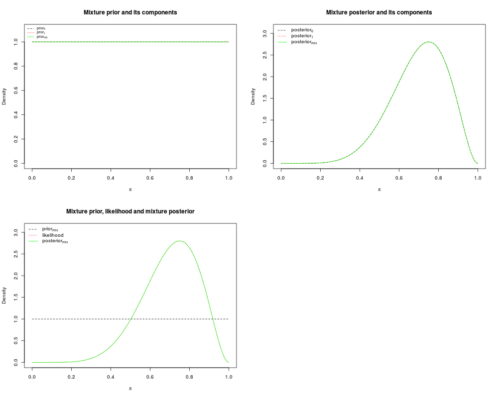
## simplest call with 6 successes observed in 8 trials and a 50:50 mix
## of two beta(1,1) uniform priors
binomixp(6,8)
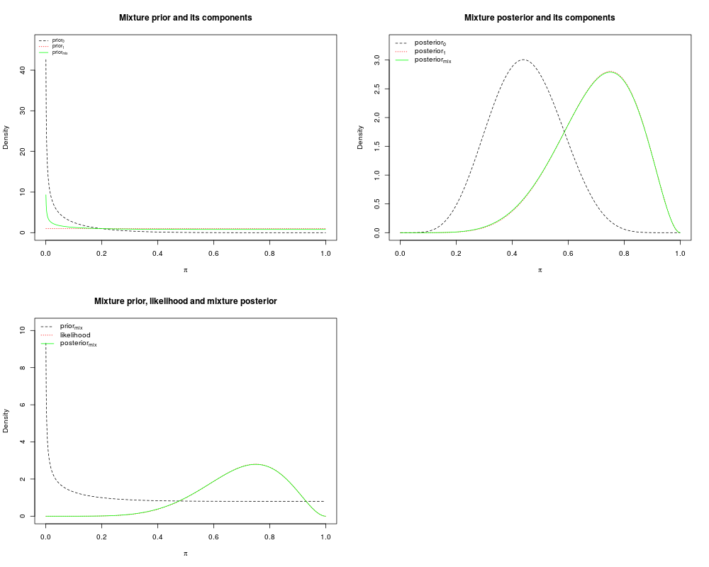
## 6 successes observed in 8 trials and a 20:80 mix of a non-uniform
## beta(0.5,6) prior and a uniform beta(1,1) prior
binomixp(6,8,alpha0=c(0.5,6),alpha1=c(1,1),p=0.2)
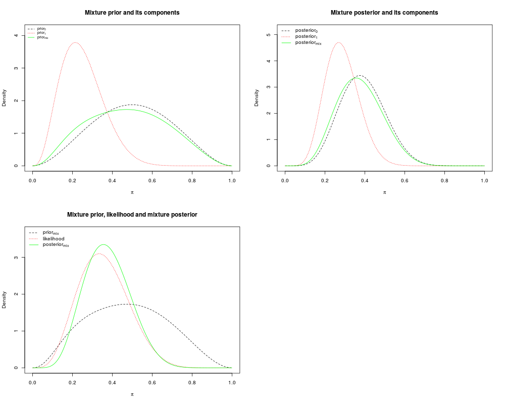
## 4 successes observed in 12 trials with a 90:10 non uniform beta(3,3) prior
## and a non uniform beta(4,12).
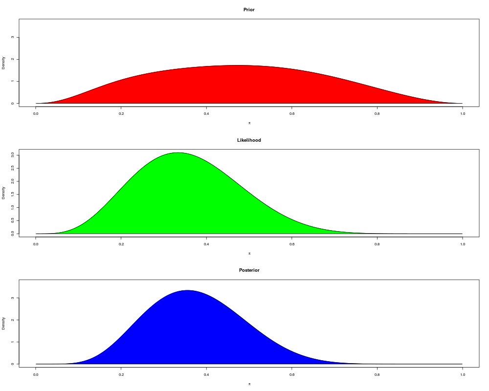
## Plot the stored prior, likelihood and posterior
results = binomixp(4,12,c(3,3),c(4,12),0.9)$mix
par(mfrow=c(3,1))
y.lims = c(0,1.1*max(results$posterior,results$prior))
plot(results$pi,results$prior,ylim=y.lims,type="l"
,xlab=expression(pi),ylab="Density",main="Prior")
polygon(results$pi,results$prior,col="red")
plot(results$pi,results$likelihood,type="l"
,xlab=expression(pi),ylab="Density",main="Likelihood")
polygon(results$pi,results$likelihood,col="green")
plot(results$pi,results$posterior,ylim=y.lims,type="l"
,xlab=expression(pi),ylab="Density",main="Posterior")
polygon(results$pi,results$posterior,col="blue")
Results
R version 3.3.1 (2016-06-21) -- "Bug in Your Hair"
Copyright (C) 2016 The R Foundation for Statistical Computing
Platform: x86_64-pc-linux-gnu (64-bit)

R is free software and comes with ABSOLUTELY NO WARRANTY.
You are welcome to redistribute it under certain conditions.
Type 'license()' or 'licence()' for distribution details.

R is a collaborative project with many contributors.
Type 'contributors()' for more information and
'citation()' on how to cite R or R packages in publications.

Type 'demo()' for some demos, 'help()' for on-line help, or
'help.start()' for an HTML browser interface to help.
Type 'q()' to quit R.

> library(Bolstad)

Attaching package: 'Bolstad'

The following objects are masked from 'package:stats':

    IQR, sd, var

> png(filename="/home/ddbj/snapshot/RGM3/R_CC/result/Bolstad/binomixp.Rd_%03d_medium.png", width=480, height=480)
> ### Name: binomixp
> ### Title: Binomial sampling with a beta mixture prior
> ### Aliases: binomixp
> ### Keywords: misc
>
> ### ** Examples
>
>
> ## simplest call with 6 successes observed in 8 trials and a 50:50 mix
> ## of two beta(1,1) uniform priors
> binomixp(6,8)
Prior probability of the data under component 0
----------------------------
Log prob.:	 -2.2
Probability:	  0.11111

Prior probability of the data under component 1
----------------------------
Log prob.:	 -2.2
Probability:	  0.11111

Post. mixing proportion for component 0:	 0.5
Post. mixing proportion for component 1:	 0.5
>
> ## 6 successes observed in 8 trials and a 20:80 mix of a non-uniform
> ## beta(0.5,6) prior and a uniform beta(1,1) prior
> binomixp(6,8,alpha0=c(0.5,6),alpha1=c(1,1),p=0.2)
Prior probability of the data under component 0
----------------------------
Log prob.:	 -6.04
Probability:	  0.0023812

Prior probability of the data under component 1
----------------------------
Log prob.:	 -2.2
Probability:	  0.11111

Post. mixing proportion for component 0:	 0.00533
Post. mixing proportion for component 1:	 0.995
>
> ## 4 successes observed in 12 trials with a 90:10 non uniform beta(3,3) prior
> ## and a non uniform beta(4,12).
> ## Plot the stored prior, likelihood and posterior
> results = binomixp(4,12,c(3,3),c(4,12),0.9)$mix
Prior probability of the data under component 0
----------------------------
Log prob.:	 -2.22
Probability:	  0.10908

Prior probability of the data under component 1
----------------------------
Log prob.:	 -1.88
Probability:	  0.15217

Post. mixing proportion for component 0:	 0.866
Post. mixing proportion for component 1:	 0.134
>
> par(mfrow=c(3,1))
> y.lims = c(0,1.1*max(results$posterior,results$prior))
>
> plot(results$pi,results$prior,ylim=y.lims,type="l"
+ 	,xlab=expression(pi),ylab="Density",main="Prior")
> polygon(results$pi,results$prior,col="red")
>
> plot(results$pi,results$likelihood,type="l"
+ 	,xlab=expression(pi),ylab="Density",main="Likelihood")
> polygon(results$pi,results$likelihood,col="green")
>
> plot(results$pi,results$posterior,ylim=y.lims,type="l"
+ 	,xlab=expression(pi),ylab="Density",main="Posterior")
> polygon(results$pi,results$posterior,col="blue")
>
>
>
>
>
>
>
>
>
> dev.off()
null device
          1
>
 .
.