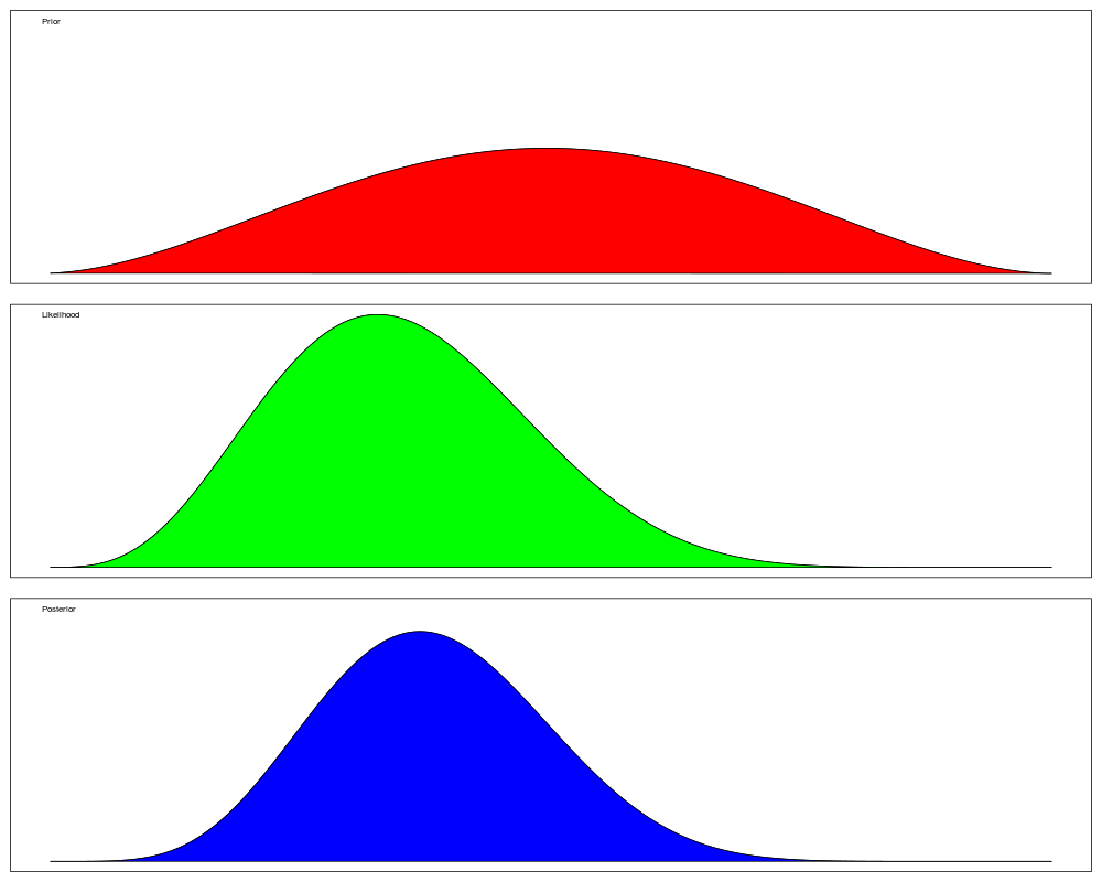
Plot the prior, likelihood, and posterior on the same plot.

Description

This function takes any object of class Bolstad and plots the prior, likelihood and posterior on the same plot. The aim is to show the influence of the prior, and the likelihood on the posterior.

Usage

decomp(x, ...)

Arguments

Note

Note that xlab, ylab, main, axes, xlim, ylim and type are all used in the function so specifying them is unlikely to have any effect.

Author(s)

James Curran

Examples

# an example with a binomial sampling situation
results = binobp(4, 12, 3, 3, plot = FALSE)
decomp(results)

# an example with normal data
y = c(2.99,5.56,2.83,3.47)
results = normnp(y, 3, 2, 1, plot = FALSE)
decomp(results)

Results

R version 3.3.1 (2016-06-21) -- "Bug in Your Hair"
Copyright (C) 2016 The R Foundation for Statistical Computing
Platform: x86_64-pc-linux-gnu (64-bit)

R is free software and comes with ABSOLUTELY NO WARRANTY.
You are welcome to redistribute it under certain conditions.
Type 'license()' or 'licence()' for distribution details.

R is a collaborative project with many contributors.
Type 'contributors()' for more information and
'citation()' on how to cite R or R packages in publications.

Type 'demo()' for some demos, 'help()' for on-line help, or
'help.start()' for an HTML browser interface to help.
Type 'q()' to quit R.

> library(Bolstad)

Attaching package: 'Bolstad'

The following objects are masked from 'package:stats':

    IQR, sd, var

> png(filename="/home/ddbj/snapshot/RGM3/R_CC/result/Bolstad/decomp.Rd_%03d_medium.png", width=480, height=480)
> ### Name: decomp
> ### Title: Plot the prior, likelihood, and posterior on the same plot.
> ### Aliases: decomp
> ### Keywords: plots
> 
> ### ** Examples
> 
> 
> # an example with a binomial sampling situation
> results = binobp(4, 12, 3, 3, plot = FALSE)
Posterior Mean           :  0.3888889 
Posterior Variance       :  0.0125081 
Posterior Std. Deviation :  0.1118397 

Prob.	Quantile 
------	---------
0.005	0.1370832
0.010	0.1552348
0.025	0.1844370
0.050	0.2119082
0.500	0.3846872
0.950	0.5802946
0.975	0.6167163
0.990	0.6577095
0.995	0.6845936
> decomp(results)
> 
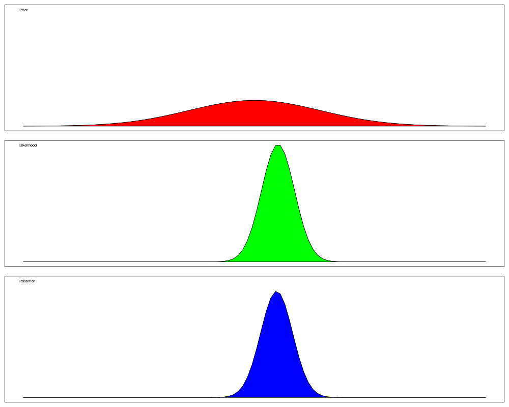
> # an example with normal data
> y = c(2.99,5.56,2.83,3.47)
> results = normnp(y, 3, 2, 1, plot = FALSE)
Known standard deviation :1
Posterior mean           : 3.6705882
Posterior std. deviation : 0.4850713

Prob.	Quantile 
------	----------
0.005	 2.4211275
0.010	 2.5421438
0.025	 2.7198661
0.050	 2.8727170
0.500	 3.6705882
0.950	 4.4684594
0.975	 4.6213104
0.990	 4.7990327
0.995	 4.9200490
> decomp(results)
> 
> 
> 
> 
> 
> 
> dev.off()
null device 
          1 
>