the rate parameter of the gamma prior. Note that the scale
is 1 / rate
scale
the scale parameter of the gamma prior
plot
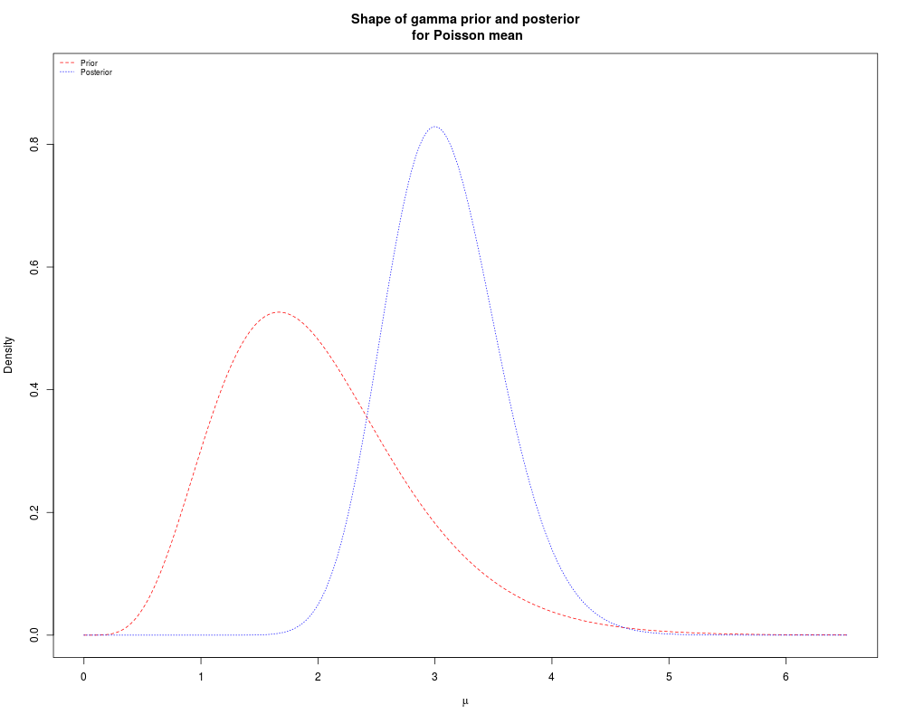
if TRUE then a plot showing the prior and the posterior
will be produced.
suppressOutput
if TRUE then none of the output is printed to
console
Value
An object of class 'Bolstad' is returned. This is a list with the
following components:
prior
the prior density assigned to mu
likelihood
the scaled likelihood function for mu given
y
posterior
the posterior probability of mu given
y
shape
the shape parameter for the gamma posterior
rate
the rate parameter for the gamma posterior
See Also
poisdppoisgcp
Examples
## simplest call with an observation of 4 and a gamma(1,1), i.e. an exponential prior on the
## mu
poisgamp(4,1,1)

##  Same as the previous example but a gamma(10,1) prior
poisgamp(4,10,1)

##  Same as the previous example but an improper gamma(1,0) prior
poisgamp(4,1,0)

## A random sample of 50 observations from a Poisson distribution with
## parameter mu = 3 and  gamma(6,3) prior
y = rpois(50,3)
poisgamp(y,6,3)

## In this example we have a random sample from a Poisson distribution
## with an unknown mean. We will use a gamma(6,3) prior to obtain the
## posterior gamma distribution, and use the R function qgamma to get a
## 95% credible interval for mu
y = c(3,4,4,3,3,4,2,3,1,7)
results = poisgamp(y,6,3)
ci = qgamma(c(0.025,0.975),results$shape, results$rate)
cat(paste("95% credible interval for mu: [",round(ci[1],3), ",", round(ci[2],3)),"]\n")

## In this example we have a random sample from a Poisson distribution
## with an unknown mean. We will use a gamma(6,3) prior to obtain the
## posterior gamma distribution, and use the R function qgamma to get a
## 95% credible interval for mu
y = c(3,4,4,3,3,4,2,3,1,7)
results = poisgamp(y, 6, 3)
ci = quantile(results, c(0.025, 0.975))
cat(paste("95% credible interval for mu: [",round(ci[1],3), ",", round(ci[2],3)),"]\n")
Results
R version 3.3.1 (2016-06-21) -- "Bug in Your Hair"
Copyright (C) 2016 The R Foundation for Statistical Computing
Platform: x86_64-pc-linux-gnu (64-bit)
R is free software and comes with ABSOLUTELY NO WARRANTY.
You are welcome to redistribute it under certain conditions.
Type 'license()' or 'licence()' for distribution details.
R is a collaborative project with many contributors.
Type 'contributors()' for more information and
'citation()' on how to cite R or R packages in publications.
Type 'demo()' for some demos, 'help()' for on-line help, or
'help.start()' for an HTML browser interface to help.
Type 'q()' to quit R.
> library(Bolstad)
Attaching package: 'Bolstad'
The following objects are masked from 'package:stats':
IQR, sd, var
> png(filename="/home/ddbj/snapshot/RGM3/R_CC/result/Bolstad/poisgamp.Rd_%03d_medium.png", width=480, height=480)
> ### Name: poisgamp
> ### Title: Poisson sampling with a gamma prior
> ### Aliases: poisgamp
> ### Keywords: misc
>
> ### ** Examples
>
>
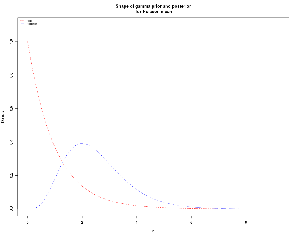
> ## simplest call with an observation of 4 and a gamma(1,1), i.e. an exponential prior on the
> ## mu
> poisgamp(4,1,1)
Summary statistics for data
---------------------------
Number of observations: 1
Sum of observations: 4
Summary statistics for posterior
--------------------------------
Shape parameter r: 5
Rate parameter v: 2
99% credible interval for mu: [ 0.54 , 6.3 ]
>
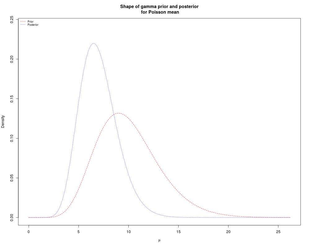
> ## Same as the previous example but a gamma(10,1) prior
> poisgamp(4,10,1)
Summary statistics for data
---------------------------
Number of observations: 1
Sum of observations: 4
Summary statistics for posterior
--------------------------------
Shape parameter r: 14
Rate parameter v: 2
99% credible interval for mu: [ 3.12 , 12.75 ]
>
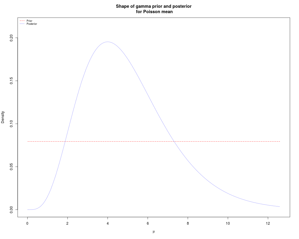
> ## Same as the previous example but an improper gamma(1,0) prior
> poisgamp(4,1,0)
Summary statistics for data
---------------------------
Number of observations: 1
Sum of observations: 4
Summary statistics for posterior
--------------------------------
Shape parameter r: 5
Rate parameter v: 1
99% credible interval : [ 1.08 , 12.59 ]
>
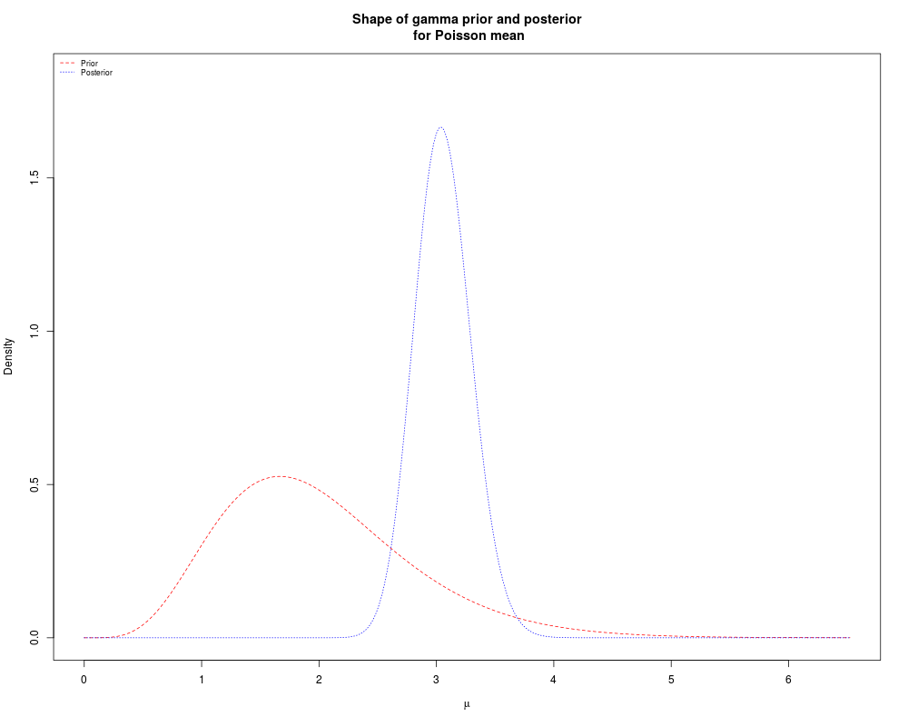
> ## A random sample of 50 observations from a Poisson distribution with
> ## parameter mu = 3 and gamma(6,3) prior
> y = rpois(50,3)
> poisgamp(y,6,3)
Summary statistics for data
---------------------------
Number of observations: 50
Sum of observations: 158
Summary statistics for posterior
--------------------------------
Shape parameter r: 164
Rate parameter v: 53
99% credible interval for mu: [ 2.51 , 3.75 ]
>
> ## In this example we have a random sample from a Poisson distribution
> ## with an unknown mean. We will use a gamma(6,3) prior to obtain the
> ## posterior gamma distribution, and use the R function qgamma to get a
> ## 95% credible interval for mu
> y = c(3,4,4,3,3,4,2,3,1,7)
> results = poisgamp(y,6,3)
Summary statistics for data
---------------------------
Number of observations: 10
Sum of observations: 34
Summary statistics for posterior
--------------------------------
Shape parameter r: 40
Rate parameter v: 13
99% credible interval for mu: [ 1.97 , 4.47 ]
> ci = qgamma(c(0.025,0.975),results$shape, results$rate)
> cat(paste("95% credible interval for mu: [",round(ci[1],3), ",", round(ci[2],3)),"]\n")
95% credible interval for mu: [ 2.198 , 4.101 ]
>
> ## In this example we have a random sample from a Poisson distribution
> ## with an unknown mean. We will use a gamma(6,3) prior to obtain the
> ## posterior gamma distribution, and use the R function qgamma to get a
> ## 95% credible interval for mu
> y = c(3,4,4,3,3,4,2,3,1,7)
> results = poisgamp(y, 6, 3)
Summary statistics for data
---------------------------
Number of observations: 10
Sum of observations: 34
Summary statistics for posterior
--------------------------------
Shape parameter r: 40
Rate parameter v: 13
99% credible interval for mu: [ 1.97 , 4.47 ]
> ci = quantile(results, c(0.025, 0.975))
> cat(paste("95% credible interval for mu: [",round(ci[1],3), ",", round(ci[2],3)),"]\n")
95% credible interval for mu: [ 2.198 , 4.101 ]
>
>
>
>
>
>
>
> dev.off()
null device
1
>
 .
.