R: Poisson sampling with a general continuous prior
poisgcp
R Documentation
Poisson sampling with a general continuous prior
Description
Evaluates and plots the posterior density for mu, the mean rate
of occurance of an event or objects, with Poisson sampling and a general
continuous prior on mu
A random sample of one or more observations from a Poisson
distribution
density
may be one of "gamma", "normal", or "user"
params
if density is one of the parameteric forms then then a vector
of parameters must be supplied. gamma: a0,b0 normal: mean,sd
n.mu
the number of possible mu values in the prior. This
number must be greater than or equal to 100. It is ignored when
density="user".
mu
a vector of possibilities for the mean of a Poisson distribution.
This must be set if density="user".
mu.prior
the associated prior density. This must be set if
density="user".
print.sum.stat
if set to TRUE then the posterior mean, posterior
variance, and a credible interval for the mean are printed. The width of the
credible interval is controlled by the parameter alpha.
alpha
The width of the credible interval is controlled by the
parameter alpha.
plot
if TRUE then a plot showing the prior and the posterior
will be produced.
suppressOutput
if TRUE then none of the output is printed to
console
Value
A list will be returned with the following components:
mu
the
vector of possible mu values used in the prior
mu.prior
the associated probability mass for the values in
mu
likelihood
the scaled likelihood function for
mu given y
posterior
the posterior probability of
mu given y
See Also
poisdppoisgamp
Examples
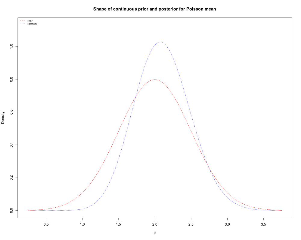
## Our data is random sample is 3, 4, 3, 0, 1. We will try a normal
## prior with a mean of 2 and a standard deviation of 0.5.
y = c(3,4,3,0,1)
poisgcp(y,density="normal",params=c(2,0.5))
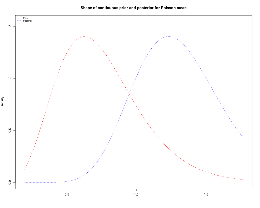
## The same data as above, but with a gamma(6,8) prior
y = c(3,4,3,0,1)
poisgcp(y,density="gamma",params=c(6,8))
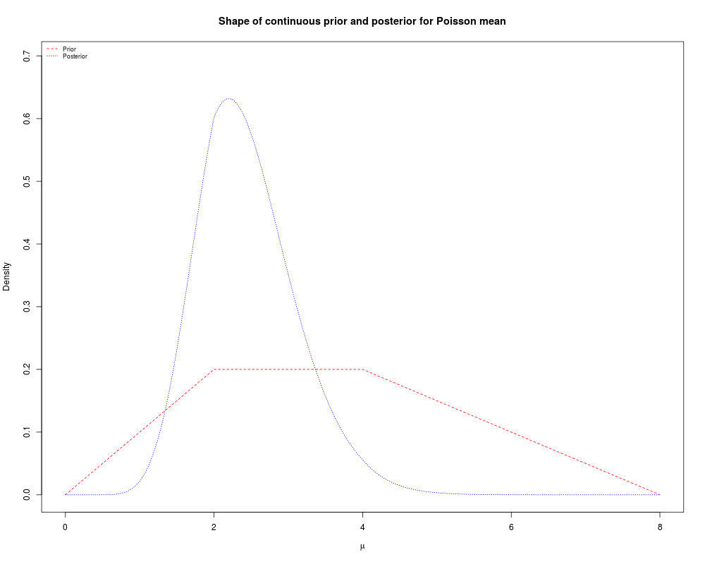
## The same data as above, but a user specified continuous prior.
## We will use print.sum.stat to get a 99% credible interval for mu.
y = c(3,4,3,0,1)
mu = seq(0,8,by=0.001)
mu.prior = c(seq(0,2,by=0.001),rep(2,1999),seq(2,0,by=-0.0005))/10
poisgcp(y,"user",mu=mu,mu.prior=mu.prior,print.sum.stat=TRUE,alpha=0.01)
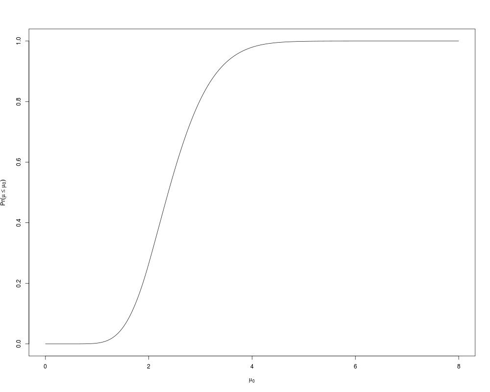
## find the posterior CDF using the results from the previous example
## and Simpson's rule. Note that the syntax of sintegral has changed.
results = poisgcp(y,"user",mu=mu,mu.prior=mu.prior)
cdf = sintegral(mu,results$posterior,n.pts=length(mu))$cdf
plot(cdf,type="l",xlab=expression(mu[0])
,ylab=expression(Pr(mu<=mu[0])))
## use the cdf to find the 95% credible region.
lcb = cdf$x[with(cdf,which.max(x[y<=0.025]))]
ucb = cdf$x[with(cdf,which.max(x[y<=0.975]))]
cat(paste("Approximate 95% credible interval : ["
,round(lcb,4)," ",round(ucb,4),"]\n",sep=""))
## find the posterior mean, variance and std. deviation
## using Simpson's rule and the output from the previous example
dens = mu*results$posterior # calculate mu*f(mu | x, n)
post.mean = sintegral(mu,dens)$value
dens = (mu-post.mean)^2*results$posterior
post.var = sintegral(mu,dens)$value
post.sd = sqrt(post.var)
# calculate an approximate 95% credible region using the posterior mean and
# std. deviation
lb = post.mean-qnorm(0.975)*post.sd
ub = post.mean+qnorm(0.975)*post.sd
cat(paste("Approximate 95% credible interval : ["
,round(lb,4)," ",round(ub,4),"]\n",sep=""))
Results
R version 3.3.1 (2016-06-21) -- "Bug in Your Hair"
Copyright (C) 2016 The R Foundation for Statistical Computing
Platform: x86_64-pc-linux-gnu (64-bit)

R is free software and comes with ABSOLUTELY NO WARRANTY.
You are welcome to redistribute it under certain conditions.
Type 'license()' or 'licence()' for distribution details.

R is a collaborative project with many contributors.
Type 'contributors()' for more information and
'citation()' on how to cite R or R packages in publications.

Type 'demo()' for some demos, 'help()' for on-line help, or
'help.start()' for an HTML browser interface to help.
Type 'q()' to quit R.

> library(Bolstad)

Attaching package: 'Bolstad'

The following objects are masked from 'package:stats':

    IQR, sd, var

> png(filename="/home/ddbj/snapshot/RGM3/R_CC/result/Bolstad/poisgcp.Rd_%03d_medium.png", width=480, height=480)
> ### Name: poisgcp
> ### Title: Poisson sampling with a general continuous prior
> ### Aliases: poisgcp
> ### Keywords: misc
>
> ### ** Examples
>
>
> ## Our data is random sample is 3, 4, 3, 0, 1. We will try a normal
> ## prior with a mean of 2 and a standard deviation of 0.5.
> y = c(3,4,3,0,1)
> poisgcp(y,density="normal",params=c(2,0.5))
Summary statistics for data
---------------------------
Number of observations:	 5
Sum of observations:	 11
>
> ## The same data as above, but with a gamma(6,8) prior
> y = c(3,4,3,0,1)
> poisgcp(y,density="gamma",params=c(6,8))
Summary statistics for data
---------------------------
Number of observations:	 5
Sum of observations:	 11
>
> ## The same data as above, but a user specified continuous prior.
> ## We will use print.sum.stat to get a 99% credible interval for mu.
> y = c(3,4,3,0,1)
> mu = seq(0,8,by=0.001)
> mu.prior = c(seq(0,2,by=0.001),rep(2,1999),seq(2,0,by=-0.0005))/10
> poisgcp(y,"user",mu=mu,mu.prior=mu.prior,print.sum.stat=TRUE,alpha=0.01)
Summary statistics for data
---------------------------
Number of observations:	 5
Sum of observations:	 11

Posterior distribution summary statistics
-----------------------------------------
Post. mean:	 2.448
Post. var.:	 0.4398
99 % cred. int.: [ 1.067 , 4.476 ]

>
> ## find the posterior CDF using the results from the previous example
> ## and Simpson's rule. Note that the syntax of sintegral has changed.
> results = poisgcp(y,"user",mu=mu,mu.prior=mu.prior)
Summary statistics for data
---------------------------
Number of observations:	 5
Sum of observations:	 11
> cdf = sintegral(mu,results$posterior,n.pts=length(mu))$cdf
> plot(cdf,type="l",xlab=expression(mu[0])
+ 	,ylab=expression(Pr(mu<=mu[0])))
>
> ## use the cdf to find the 95% credible region.
> lcb = cdf$x[with(cdf,which.max(x[y<=0.025]))]
> ucb = cdf$x[with(cdf,which.max(x[y<=0.975]))]
> cat(paste("Approximate 95% credible interval : ["
+ 	,round(lcb,4)," ",round(ucb,4),"]\n",sep=""))
Approximate 95% credible interval : [1.3373 3.925]
>
> ## find the posterior mean, variance and std. deviation
> ## using Simpson's rule and the output from the previous example
> dens = mu*results$posterior # calculate mu*f(mu | x, n)
> post.mean = sintegral(mu,dens)$value
>
> dens = (mu-post.mean)^2*results$posterior
> post.var = sintegral(mu,dens)$value
> post.sd = sqrt(post.var)
>
> # calculate an approximate 95% credible region using the posterior mean and
> # std. deviation
> lb = post.mean-qnorm(0.975)*post.sd
> ub = post.mean+qnorm(0.975)*post.sd
>
> cat(paste("Approximate 95% credible interval : ["
+ 	,round(lb,4)," ",round(ub,4),"]\n",sep=""))
Approximate 95% credible interval : [1.1482 3.7478]
>
>
>
>
>
>
> dev.off()
null device
          1
>
 .
.