CircNNTSR: An R Package for the statistical analysis of circular data using nonnegative trigonometric sums (NNTS) models

Description

A collection of utilities for the statistical analysis of circular and spherical data using nonnegative trigonometric sum (NNTS) models

Details

Fernandez-Duran, J.J. (2004) proposed a new family of distributions for circular random variables based on nonnegative trigonometric sums. This package provides functions for working with circular distributions based on nonnegative trigonometric sums, including functions for estimating the parameters and plotting the densities.

The distribution function in this package is a circular distribution based on nonnegative trigonometric sums (Fernandez-Duran, 2004). Fejer (1915) expressed a univariate nonnegative trigonometric (Fourier) sum (series), for a variable theta, as the squared modulus of a sum of complex numbers, i.e.,

||sum_{k=0}^M c_k*exp{i*k*theta}||^2 (1)

where i=sqrt(-1). From this result, the parameters (a_k,b_k) for k=1,…, M of the trigonometric sum of order M,T(theta),

T(theta)=a_0 + sum_{k=1}^M(a_k*cos(k*theta) + b_k*sin(k*theta))

are expressed in terms of the complex parameters in Equation 1 , c_k, for k=0,…, M, as a_k - i*b_k= 2*sum_{ν=0}^{n-k}c_{nu + k}*overline{c}_{ν}. The additional constraint, sum_{k=0}^n||c_k||^2=1/(2*pi)=a_0, is imposed to make the trigonometric sum to integrate one. Thus, c_0 must be real and positive, and there are 2*M free parameters. Then, the probability density function for a circular (angular) random variable is defined as (Fernandez-Duran, 2004)

f(theta; underline{a},underline{b},M)=1/(2*pi) + 1/pi*sum_{k=1}^M(a_k*cos(k*theta) + b_k*sin(k*theta)).

Note that Equation 1 can also be expressed as a double sum as

sum_{k=0}^{M}sum_{m=0}^{M}c_k*underline{c}_m*exp(i*(k-m)*theta).

The underline{c} parameters can also be expressed in polar coordinates as c_k=rho_k*exp(i*phi_k) for rho_k >= 0 and phi_k en [0,2*pi); where rho_k is the modulus of c_k and phi_k is the argument of c_k for k=1,…,M. Many functions of the packages use as parameters the squared moduli and the arguments of c_k, rho_k^2 and phi_k, for k=1,…,M. We refer to the parameter M as the number of components in the NNTS.

Author(s)

Juan Jose Fernandez-Duran and Maria Mercedes Gregorio-Dominguez

Maintainer: Maria Mercedes Gregorio Dominguez <mercedes@itam.mx>

References

Fernandez-Duran, J.J. (2004). Circular Distributions Based on Nonnegative Trigonometric Sums, Biometrics, 60(2), 499-503.

Fernandez-Duran, J.J., Gregorio-Dominguez, M.M. (2010). A Likelihood-Ratio Test for Homogeneity in Circular Data. Journal of Biometrics & Biostatistics, 1(3), 107. doi:10.4172/2155-6180.1000107

Fernandez-Duran, J.J., Gregorio-Dominguez, M.M. (2010). Maximum Likelihood Estimation of Nonnegative Trigonometric Sums Models Using a Newton-Like Algorithm on Manifolds. Electronic Journal of Statistics, 4, 1402-1410. doi:10.1214/10-ejs587

Fernandez-Duran, J.J., Gregorio-Dominguez, M.M. (2014). Distributions for Spherical Data Based on Nonnegative Trigonometric Sums. Statistical Papers, 55(4), 983-1000. doi:10.1007/s00362-013-0547-5

Fernandez-Duran, J.J., Gregorio-Dominguez, M.M. (2014). Modeling Angles in Proteins and Circular Genomes Using Multivariate Angular Distributions Based on Nonnegative Trigonometric Sums. Statistical Applications in Genetics and Molecular Biology, 13(1), 1-18. doi:10.1515/sagmb-2012-0012

Fernandez-Duran, J.J., Gregorio-Dominguez, M.M. (2014). Testing for Seasonality Using Circular Distributions Based on Nonnegative Trigonometric Sums as Alternative Hypotheses. Statistical Methods in Medical Research, 23(3), 279-292. doi:10.1177/0962280211411531.

Juan Jose Fernandez-Duran, Maria Mercedes Gregorio-Dominguez (2016). CircNNTSR: An R Package for the Statistical Analysis of Circular, Multivariate Circular, and Spherical Data Using Nonnegative Trigonometric Sums. Journal of Statistical Software, 70(6), 1-19. doi:10.18637/jss.v070.i06

Examples

a<-c(runif(10,3*pi/2,2*pi-0.00000001),runif(10,pi/2,pi-0.00000001))
#Estimation of the NNTSdensity with 2 components for data and 1000 iterations
est<-nntsmanifoldnewtonestimation(a,2,1000)
#plot the estimated density
nntsplot(est$cestimates[,2],2)

data(Turtles_radians)
#Empirical analysis of data
Turtles_hist<-hist(Turtles_radians,breaks=10,freq=FALSE)
#Estimation of the NNTS density with 3 componentes for data
est<-nntsmanifoldnewtonestimation(Turtles_radians,3)
est
#plot the estimated density
nntsplot(est$cestimates[,2],3)
#add the histogram to the estimated density plot
plot(Turtles_hist, freq=FALSE, add=TRUE)

b<-c(runif(10,3*pi/2,2*pi-0.00000001),runif(10,pi/2,pi-0.00000001))
estS<-nntsestimationSymmetric(2,b)
nntsplotSymmetric(estS$coef,2)

M<-c(2,3)
R<-length(M)
data(Nest)
data<-Nest
est<-mnntsmanifoldnewtonestimation(data,M,R,1000)
est
cest<-est$cestimates
mnntsplot(cest, M)

data(Datab6fisher_ready)
data<-Datab6fisher_ready
M<-c(4,4)
cpars<-rnorm(prod(M+1))+rnorm(prod(M+1))*complex(real=0,imaginary=1)
cpars[1]<-Re(cpars[1])
cpars<- cpars/sqrt(sum(Mod(cpars)^2))
snntsdensity(data, cpars, M)
snntsloglik(data, cpars, M)

data(Datab6fisher_ready)
data<-Datab6fisher_ready
M<-c(1,2)
cest<-snntsmanifoldnewtonestimation(data, M)
lat<-snntsmarginallatitude(seq(0,pi,.1),cest$cestimates[,3],M)
plot(seq(0,pi,.1),lat,type="l")

Results

R version 3.3.1 (2016-06-21) -- "Bug in Your Hair"
Copyright (C) 2016 The R Foundation for Statistical Computing
Platform: x86_64-pc-linux-gnu (64-bit)

R is free software and comes with ABSOLUTELY NO WARRANTY.
You are welcome to redistribute it under certain conditions.
Type 'license()' or 'licence()' for distribution details.

R is a collaborative project with many contributors.
Type 'contributors()' for more information and
'citation()' on how to cite R or R packages in publications.

Type 'demo()' for some demos, 'help()' for on-line help, or
'help.start()' for an HTML browser interface to help.
Type 'q()' to quit R.

> library(CircNNTSR)

Attaching package: 'CircNNTSR'

The following object is masked from 'package:grDevices':

    trans3d

> png(filename="/home/ddbj/snapshot/RGM3/R_CC/result/CircNNTSR/CircNNTSR-package.Rd_%03d_medium.png", width=480, height=480)
> ### Name: CircNNTSR-package
> ### Title: CircNNTSR: An R Package for the statistical analysis of circular
> ###   data using nonnegative trigonometric sums (NNTS) models
> ### Aliases: CircNNTSR-package CircNNTSR
> ### Keywords: package
> 
> ### ** Examples
> 
> a<-c(runif(10,3*pi/2,2*pi-0.00000001),runif(10,pi/2,pi-0.00000001))
> #Estimation of the NNTSdensity with 2 components for data and 1000 iterations
> est<-nntsmanifoldnewtonestimation(a,2,1000)
> #plot the estimated density
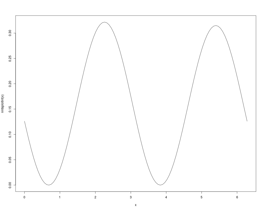
> nntsplot(est$cestimates[,2],2)
> 
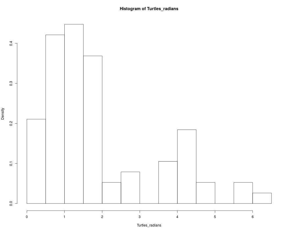
> data(Turtles_radians)
> #Empirical analysis of data
> Turtles_hist<-hist(Turtles_radians,breaks=10,freq=FALSE)
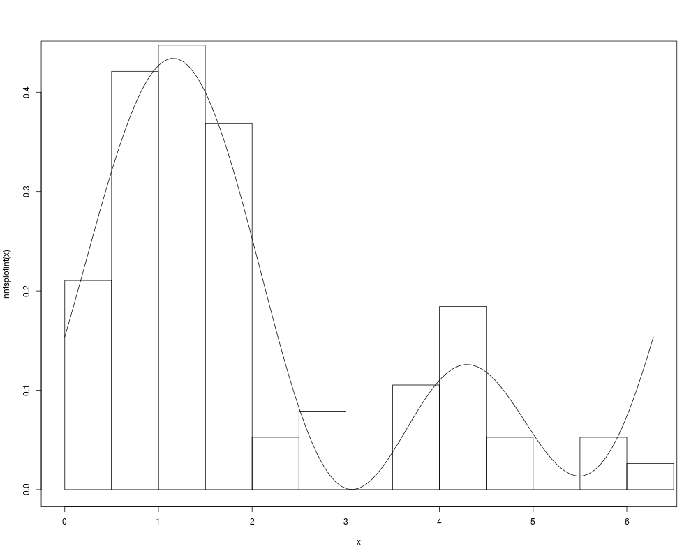
> #Estimation of the NNTS density with 3 componentes for data
> est<-nntsmanifoldnewtonestimation(Turtles_radians,3)
> est
$cestimates
  k              cestimates
1 0  0.28645175+0.00000000i
2 1  0.11655438-0.12669303i
3 2 -0.14659000-0.16080633i
4 3  0.01079598+0.00065866i

$loglik
[1] -107.9374

$AIC
[1] 227.8749

$BIC
[1] 241.8593

$gradnormerror
[1] 2.466083e-08

> #plot the estimated density
> nntsplot(est$cestimates[,2],3)
> #add the histogram to the estimated density plot
> plot(Turtles_hist, freq=FALSE, add=TRUE)
> 
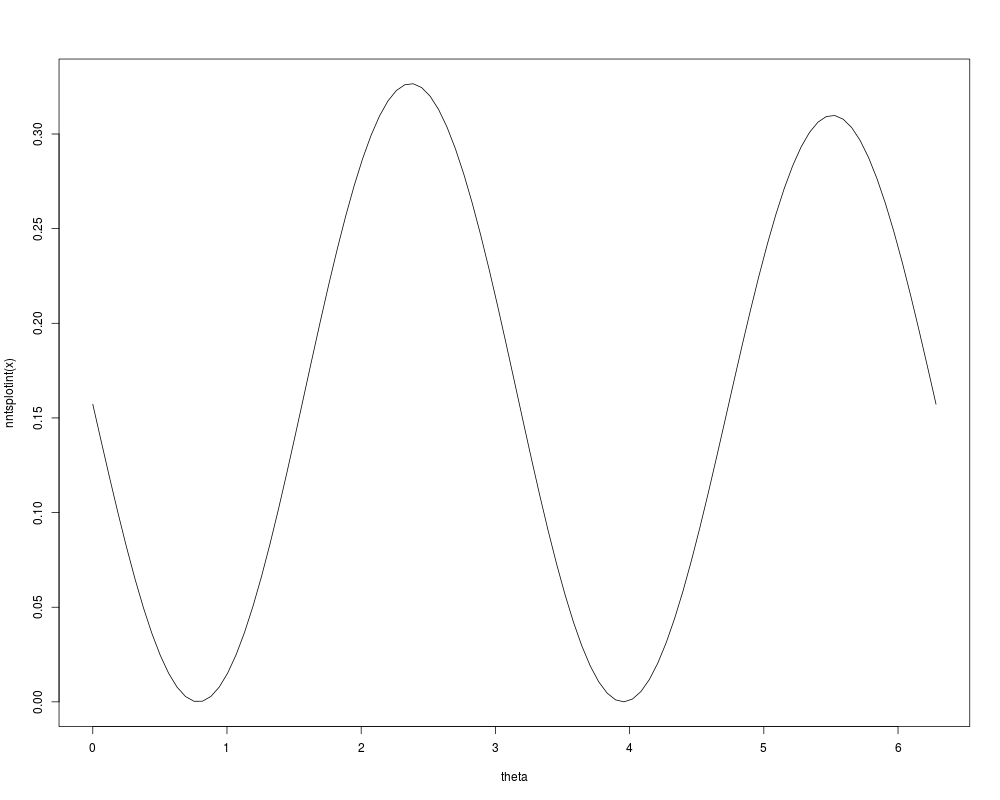
> b<-c(runif(10,3*pi/2,2*pi-0.00000001),runif(10,pi/2,pi-0.00000001))
> estS<-nntsestimationSymmetric(2,b)
> nntsplotSymmetric(estS$coef,2)
> 
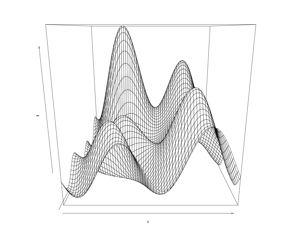
> M<-c(2,3)
> R<-length(M)
> data(Nest)
> data<-Nest
> est<-mnntsmanifoldnewtonestimation(data,M,R,1000)
> est
$cestimates
   1 2                cestimates
1  0 0  0.129365319+0.000000000i
2  1 0 -0.022724537+0.030193689i
3  2 0 -0.041968214+0.017942911i
4  0 1  0.027583559+0.028548740i
5  1 1  0.017872338-0.019121344i
6  2 1 -0.021294780-0.006160541i
7  0 2 -0.001282377+0.009097531i
8  1 2  0.008477646-0.020693765i
9  2 2 -0.000597991+0.008993618i
10 0 3 -0.024891098+0.004757459i
11 1 3 -0.010734043+0.021830576i
12 2 3  0.016843000+0.012156602i

$loglik
[1] -170.9465

$AIC
[1] 385.8931

$BIC
[1] 427.9576

$gradnormerror
[1] 2.75761e-16

> cest<-est$cestimates
> mnntsplot(cest, M)
> 
> data(Datab6fisher_ready)
> data<-Datab6fisher_ready
> M<-c(4,4)
> cpars<-rnorm(prod(M+1))+rnorm(prod(M+1))*complex(real=0,imaginary=1)
> cpars[1]<-Re(cpars[1])
> cpars<- cpars/sqrt(sum(Mod(cpars)^2))
> snntsdensity(data, cpars, M)
              [,1]
  [1,] 0.032678547
  [2,] 0.037269499
  [3,] 0.058525540
  [4,] 0.053936297
  [5,] 0.074047611
  [6,] 0.078706233
  [7,] 0.037829444
  [8,] 0.096171585
  [9,] 0.096031604
 [10,] 0.035592552
 [11,] 0.052978877
 [12,] 0.079201554
 [13,] 0.030873761
 [14,] 0.064656429
 [15,] 0.071244453
 [16,] 0.069673940
 [17,] 0.020070942
 [18,] 0.081322844
 [19,] 0.052906357
 [20,] 0.063820124
 [21,] 0.117575006
 [22,] 0.060557801
 [23,] 0.070024439
 [24,] 0.056558930
 [25,] 0.056010120
 [26,] 0.117447591
 [27,] 0.101817923
 [28,] 0.062884404
 [29,] 0.030836763
 [30,] 0.021728491
 [31,] 0.115024804
 [32,] 0.017612059
 [33,] 0.051259859
 [34,] 0.114579781
 [35,] 0.115752132
 [36,] 0.050742616
 [37,] 0.003092554
 [38,] 0.035817723
 [39,] 0.058746129
 [40,] 0.039599866
 [41,] 0.060679969
 [42,] 0.016953817
 [43,] 0.031360942
 [44,] 0.071167325
 [45,] 0.109143647
 [46,] 0.067990599
 [47,] 0.054558889
 [48,] 0.116468502
 [49,] 0.108956316
 [50,] 0.104246980
 [51,] 0.083403419
 [52,] 0.094662415
 [53,] 0.106222130
 [54,] 0.064992476
 [55,] 0.099843735
 [56,] 0.067032905
 [57,] 0.070935649
 [58,] 0.011384557
 [59,] 0.041053827
 [60,] 0.029803149
 [61,] 0.070374839
 [62,] 0.085317673
 [63,] 0.070024713
 [64,] 0.079678164
 [65,] 0.094663297
 [66,] 0.066131966
 [67,] 0.073211546
 [68,] 0.044702846
 [69,] 0.010545717
 [70,] 0.078725435
 [71,] 0.053148279
 [72,] 0.075022256
 [73,] 0.009387842
 [74,] 0.025606634
 [75,] 0.053224888
 [76,] 0.056495629
 [77,] 0.068333653
 [78,] 0.088134416
 [79,] 0.043472437
 [80,] 0.022620868
 [81,] 0.021800350
 [82,] 0.029368215
 [83,] 0.082312556
 [84,] 0.058802035
 [85,] 0.063615248
 [86,] 0.034000532
 [87,] 0.052752235
 [88,] 0.036290223
 [89,] 0.022461741
 [90,] 0.051866579
 [91,] 0.045236906
 [92,] 0.050919607
 [93,] 0.056286535
 [94,] 0.069205749
 [95,] 0.049581910
 [96,] 0.038988177
 [97,] 0.057336735
 [98,] 0.074133001
 [99,] 0.041462930
[100,] 0.046801122
[101,] 0.050038470
[102,] 0.042063549
[103,] 0.058698942
[104,] 0.056860748
[105,] 0.084450707
[106,] 0.072366765
[107,] 0.023283021
> snntsloglik(data, cpars, M)
[1] -315.6245
> 
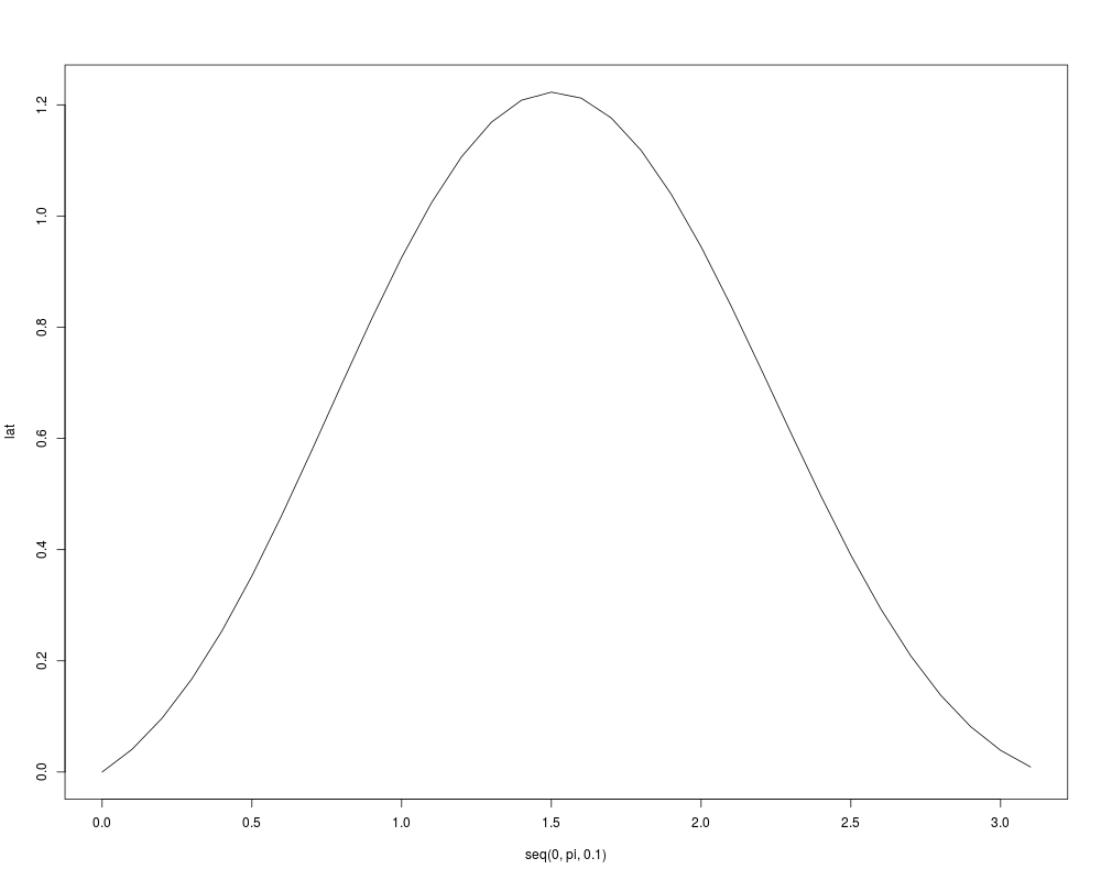
> data(Datab6fisher_ready)
> data<-Datab6fisher_ready
> M<-c(1,2)
> cest<-snntsmanifoldnewtonestimation(data, M)
> lat<-snntsmarginallatitude(seq(0,pi,.1),cest$cestimates[,3],M)
> plot(seq(0,pi,.1),lat,type="l")
> 
> 
> 
> 
> 
> 
> 
> dev.off()
null device 
          1 
>