R Graphical Manual

Browse All

Last data update: 2014.03.03

R: DBChIP

DBChIP

R Documentation

DBChIP

Description

Detecting differential binding of transcription factors with ChIP-seq

Usage

DBChIP(binding.site.list, chip.data.list, conds, input.data.list = NULL,
 data.type = c("MCS", "AlignedRead", "BED"), frag.len = 200, chr.vec = NULL, 
 chr.exclusion = NULL, chr.len.vec = NULL, subtract.input = FALSE, norm.factor.vec = NULL, 
 in.distance = 100, out.distance = 250, window.size = 250,
 dispersion=NULL, common.disp=TRUE, prior.n=10, 
 two.sample.method="composite.null", allowable.FC=1.5, collapsed.quant=0.5)

Arguments

`binding.site.list`	a list of data.frames. Each data.frame corresponds to one condition in comparison and has three fields, chr, pos, and weight, to indicate the binding location and strength.
`chip.data.list`	a list of ChIP data where each list item corresponds to one ChIP library. The name of the items should be unique. Biological replicates should be in separate items. Each item can be one of three accepted data types: MCS, AlignedRead and BED.
`conds`	a vector of conditions of ChIP libraries. Should be the same order as chip.data.list, or the names should be specified as a permutation of the names of chip.data.list.
`input.data.list`	a list of control data. Should have same data type as in chip.data.list. The names of the items should be unique, and each name should be matched to either a ChIP replicate name when the two are paired or a condition name in general.
`data.type`	"MCS", "AlignedRead" or "BED". See Details.
`frag.len`	average fragment length. Default 200 bp.
`chr.vec`	a vector of chromosomes in data. User can specify chr.vec, or it can be computed from the ChIP and control samples.
`chr.exclusion`	user can either specify chr.vec, or specify the chromosomes to exclude through this parameter.
`chr.len.vec`	a vector of chromosome lengths corresponding to chr.vec. Can be specified if known, or will be computed as the largest 5' end position in the data.
`subtract.input`	logical. Whether input will be subtracted from ChIP when counting the binding reads. Default is FALSE.
`norm.factor.vec`	a vector of normalization factors between the ChIP and control libraries when controls are available. Can be specified, or will be computed by DBChIP.
`in.distance`	within cluster distance. If the distance between centroids of two clusters are smaller than this value, the clusters will be merged into one. Default value 100 bp.
`out.distance`	out of cluster distance. If the distance between centroids of two clusters are larger than this value, they are considered different binding sites. Also double-function as the window size to count reads around each site. Default value 250 bp.
`window.size`	the window size to count reads around a binding site.
`dispersion`	The dispersion parameter in Negative Binomial distribution. Could be a numerical value or a vector with a length of the number of consensus sites.
`common.disp`	logical, TRUE (use common dispersion parameter for all sites) or FALSE (use site-specific dispersion).
`prior.n`	a parameter regulate the degree of pooling when using site-specific dispersion (`common.disp`=FALSE).
`two.sample.method`	the method to use when comparing two condition with no replicates. The default is to test a composite null that allow certain fold change `allowable.FC`. Otherwise user should provide a dispersion parameter.
`allowable.FC`	allowable fold change when testing a composite null. Default value 1.5.
`collapsed.quant`	the quantile to use when testing more than two conditions without replicates. Default value is 0.5, the median.

Details

The ChIP and control data should be properly filtered before the analysis to avoid artifacts. For example, reads mapping to mitochondrial DNA, or Y chromosome for female samples will need to be filtered.

Filtering of chromosomes can be achieved through specification of chr.vec and/or chr.exclusion. Only reads from chromosomes in chr.vec but not in chr.exclusion are utilized in the analysis.

User can include or exclude sex chromosomes in the computation, depending on whether protein-DNA bindings on sex chromosomes are of research interest.

Biological replicates of a ChIP sample should be kept separate so that dispersion can be properly estimated. On the other hand, replicates of a control/input sample should be merged because the purpose of the control samples is to estimate the background for testing and plotting. One exception would be when a control replicate is paired with a ChIP replicate, for example, they are coming from the same batch, a portion of which is used for IP and the other portion is used for control. In such case, the control replicate can be kept separate with the same name of the matching ChIP replicate.

data.type

MCS Minimum ChIP-Seq format. data.frame with fields: chr (factor), pos (integer) and strand (factor, "+" and "-"). pos is 5' location. This is different from eland default which use 3' location for reverse strand.
AlignedRead from Bioconductor ShortRead package (with support of commonly used formats, including Eland, MAQ, Bowtie, SOAP and BAM).
BED with at least first 6 fields (chrom, start, end, name, score and strand), http://genome.ucsc.edu/FAQ/FAQformat.html#format1.

Users are recommended to study the histogram of the $p$-values for model checking. More specifically, the $p$-values between 0.5 and 1 should be roughly uniform. When many replicates are available, users can also randomly split biological replicates of the same condition and perform comparisons through DBChIP using the estimated dispersion parameter to check whether the $p$-values look uniform.

Value

A list with following components:

`chip.list`	the list of ChIP data in internal MCS format.
`conds`	vector of conditions of ChIP libraries.
`frag.len`	average fragment length.
`chr.vec`	a vector of chromosomes in data.
`chr.len.vec`	a vector of chromosome lengths corresponding to chr.vec.
`consensus.site`	consensus sites. It is a data.frame, for details, see `site.merge`.
`site.count`	a data.frame of read counts at each consensus site.
`test.stat`	a data.frame of test statistics for testing non-differential binding at each site, include p-values and fold changes.
`input.list`	the list of control data. The components from this and below are only available when control data are available.
`matching.input.names`	the matching input names for ChIP libraries.
`norm.factor.vec`	vector of normalization factors between the ChIP and control libraries when controls are available. Can be specified, or will be computed by DBChIP.

Author(s)

Kun Liang, kliang@stat.wisc.edu

References

Liang, K and Keles, S (2012). Detecting differential binding of transcription factors with ChIP-seq. Bioinformatics, 28, 121-122.

Examples

data("PHA4")
dat <- DBChIP(binding.site.list, chip.data.list=chip.data.list, input.data.list=input.data.list, conds=conds, data.type="MCS")
rept <- report.peak(dat)
rept
#pdf("Diff.Binding.pdf")
plotPeak(rept, dat)
#dev.off()

## experienced users can proceed in a step by step fashion such that if program
## needs to be run for a different setting, intermediate results can be saved and reused.
data("PHA4")
conds <- factor(c("emb","emb","L1", "L1"), levels=c("emb", "L1"))

bs.list <- read.binding.site.list(binding.site.list)

## compute consensus site
consensus.site <- site.merge(bs.list, in.distance=100, out.distance=250)

dat <- load.data(chip.data.list=chip.data.list, conds=conds, consensus.site=consensus.site, input.data.list=input.data.list, data.type="MCS")

## count ChIP reads around each binding site
dat <- get.site.count(dat, window.size=250)

## test for differential binding
dat <- test.diff.binding(dat)

# report test result and plot the coverage profiles
rept <- report.peak(dat)
rept
plotPeak(rept, dat)

Results


R version 3.3.1 (2016-06-21) -- "Bug in Your Hair"
Copyright (C) 2016 The R Foundation for Statistical Computing
Platform: x86_64-pc-linux-gnu (64-bit)

R is free software and comes with ABSOLUTELY NO WARRANTY.
You are welcome to redistribute it under certain conditions.
Type 'license()' or 'licence()' for distribution details.

R is a collaborative project with many contributors.
Type 'contributors()' for more information and
'citation()' on how to cite R or R packages in publications.

Type 'demo()' for some demos, 'help()' for on-line help, or
'help.start()' for an HTML browser interface to help.
Type 'q()' to quit R.

> library(DBChIP)
Loading required package: edgeR
Loading required package: limma
Loading required package: DESeq
Loading required package: BiocGenerics
Loading required package: parallel

Attaching package: 'BiocGenerics'

The following objects are masked from 'package:parallel':

    clusterApply, clusterApplyLB, clusterCall, clusterEvalQ,
    clusterExport, clusterMap, parApply, parCapply, parLapply,
    parLapplyLB, parRapply, parSapply, parSapplyLB

The following object is masked from 'package:limma':

    plotMA

The following objects are masked from 'package:stats':

    IQR, mad, xtabs

The following objects are masked from 'package:base':

    Filter, Find, Map, Position, Reduce, anyDuplicated, append,
    as.data.frame, cbind, colnames, do.call, duplicated, eval, evalq,
    get, grep, grepl, intersect, is.unsorted, lapply, lengths, mapply,
    match, mget, order, paste, pmax, pmax.int, pmin, pmin.int, rank,
    rbind, rownames, sapply, setdiff, sort, table, tapply, union,
    unique, unsplit

Loading required package: Biobase
Welcome to Bioconductor

    Vignettes contain introductory material; view with
    'browseVignettes()'. To cite Bioconductor, see
    'citation("Biobase")', and for packages 'citation("pkgname")'.

Loading required package: locfit
locfit 1.5-9.1 	 2013-03-22
Loading required package: lattice
    Welcome to 'DESeq'. For improved performance, usability and
    functionality, please consider migrating to 'DESeq2'.
> png(filename="/home/ddbj/snapshot/RGM3/R_BC/result/DBChIP/DBChIP.Rd_%03d_medium.png", width=480, height=480)
> ### Name: DBChIP
> ### Title: DBChIP
> ### Aliases: DBChIP
> 
> ### ** Examples
> 
> data("PHA4")
> dat <- DBChIP(binding.site.list, chip.data.list=chip.data.list, input.data.list=input.data.list, conds=conds, data.type="MCS")
merging sites from different conditions to consensus sites.done
reading data...done
computing normalization factor between ChIP and control samples.done
count ChIP reads around each binding site.done
Common dispersion: 0.05915362 
> rept <- report.peak(dat)
> rept
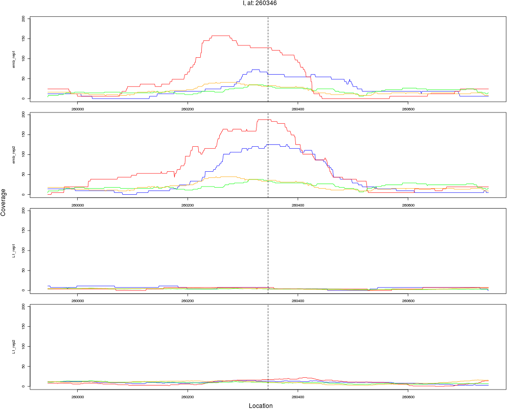
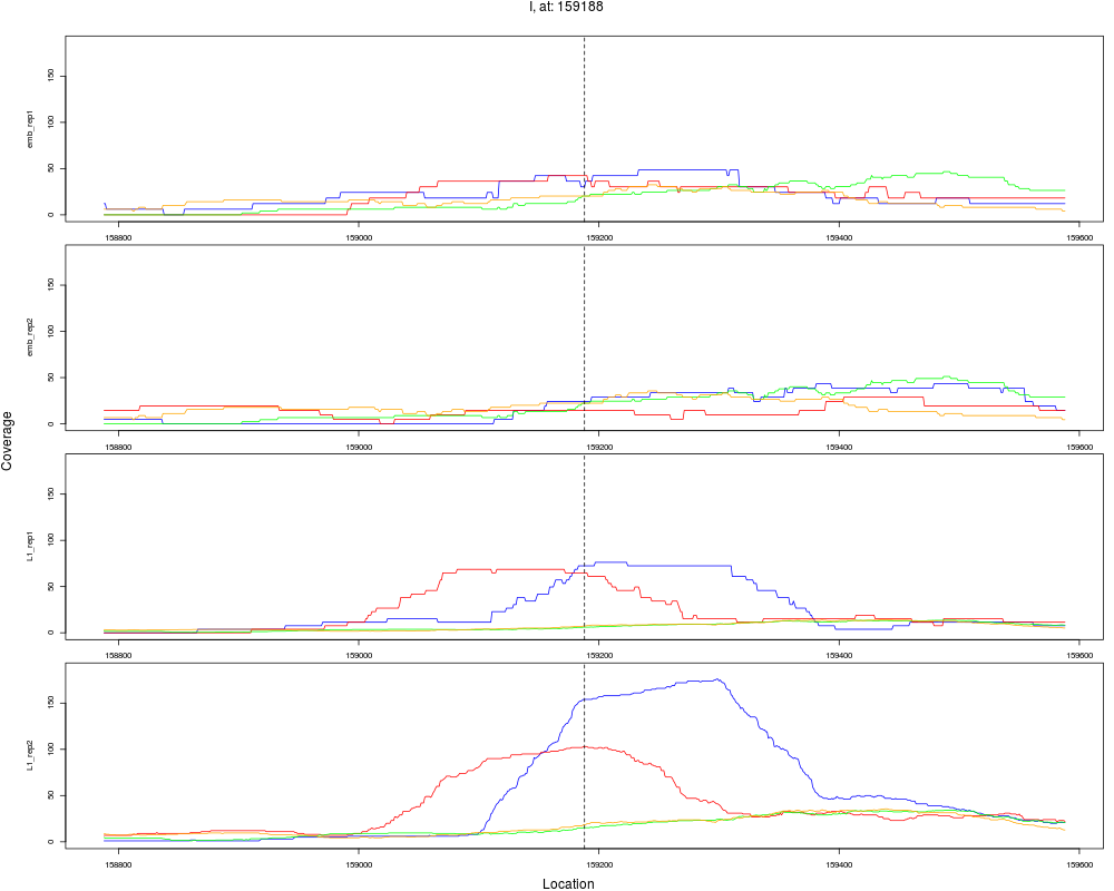
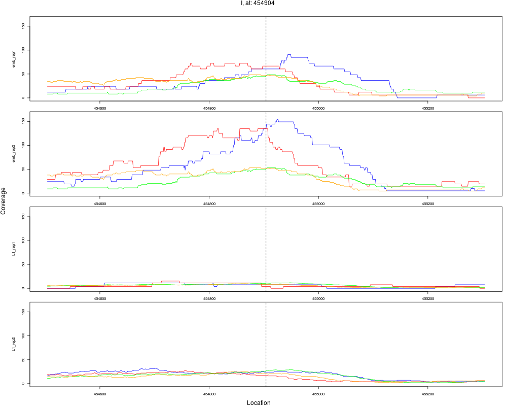
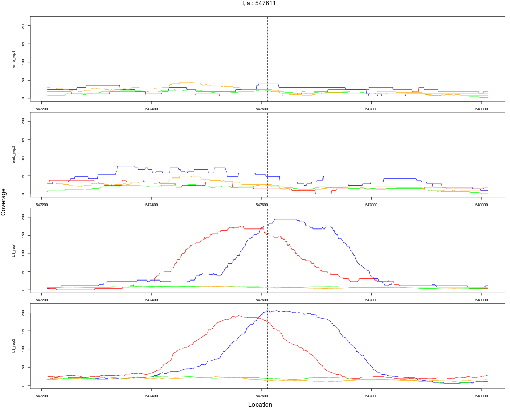
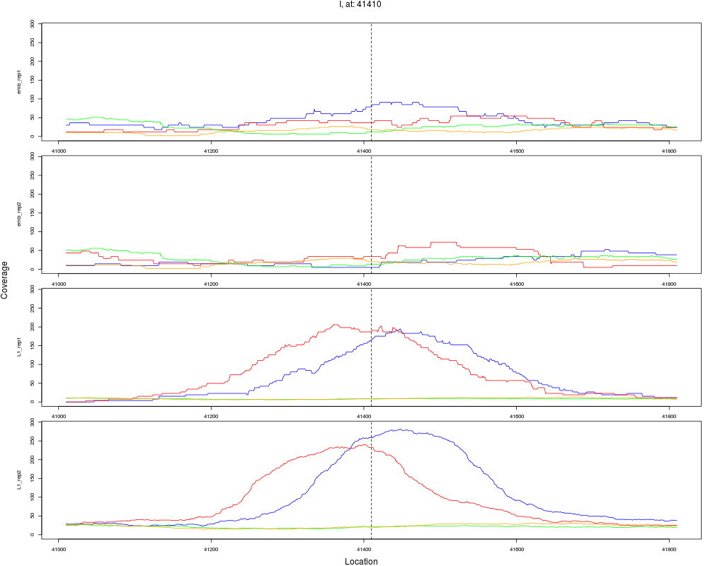
   chr    pos nsig origin ori.pos     FC.L1         pval          FDR
1    I 260346    1    emb  260346 0.1129558 1.057645e-11 5.076698e-10
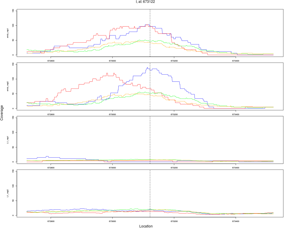
2    I 673122    1    emb  673122 0.1168590 1.798443e-10 4.316264e-09
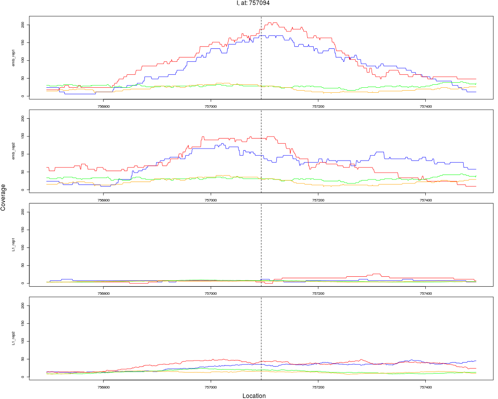
3    I 757094    1    emb  757094 0.1717831 4.012809e-09 6.420495e-08
4    I 454904    1    emb  454904 0.1632294 1.349896e-08 1.619875e-07
5    I 547611    1     L1  547611 5.6827777 2.104486e-08 2.020307e-07
6    I  41410    1     L1   41410 4.2984821 4.548449e-07 3.638759e-06
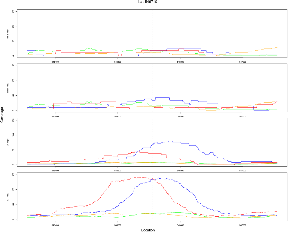
7    I 546710    1     L1  546710 4.3025538 7.621600e-06 5.226240e-05
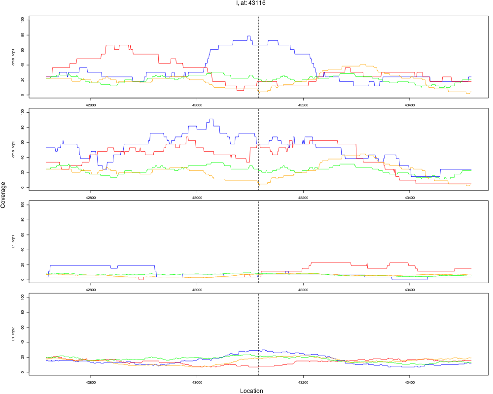
8    I  43116    1    emb   43116 0.2581921 6.466525e-05 3.879915e-04
9    I 159188    1     L1  159188 2.9888809 3.449015e-04 1.839475e-03
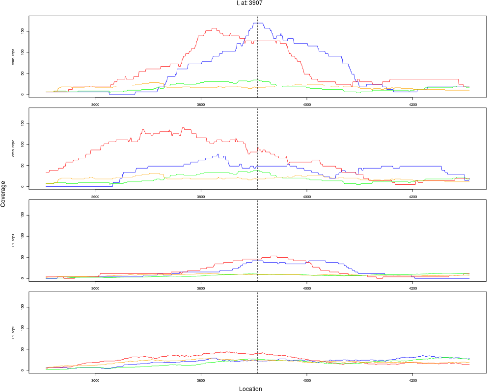
10   I   3907    1    emb    3907 0.3718658 7.035650e-04 3.377112e-03
> #pdf("Diff.Binding.pdf")
> plotPeak(rept, dat)
Warning message:
In rep(caption, length.out = nrow(rept)) :
  'x' is NULL so the result will be NULL
> #dev.off()
> 
> ## experienced users can proceed in a step by step fashion such that if program
> ## needs to be run for a different setting, intermediate results can be saved and reused.
> data("PHA4")
> conds <- factor(c("emb","emb","L1", "L1"), levels=c("emb", "L1"))
> 
> bs.list <- read.binding.site.list(binding.site.list)
> 
> ## compute consensus site
> consensus.site <- site.merge(bs.list, in.distance=100, out.distance=250)
merging sites from different conditions to consensus sites.done
> 
> dat <- load.data(chip.data.list=chip.data.list, conds=conds, consensus.site=consensus.site, input.data.list=input.data.list, data.type="MCS")
reading data...done
computing normalization factor between ChIP and control samples.done
> 
> ## count ChIP reads around each binding site
> dat <- get.site.count(dat, window.size=250)
count ChIP reads around each binding site.done
> 
> ## test for differential binding
> dat <- test.diff.binding(dat)
Common dispersion: 0.05915362 
> 
> # report test result and plot the coverage profiles
> rept <- report.peak(dat)
> rept
   chr    pos nsig origin ori.pos     FC.L1         pval          FDR
1    I 260346    1    emb  260346 0.1129558 1.057645e-11 5.076698e-10
2    I 673122    1    emb  673122 0.1168590 1.798443e-10 4.316264e-09
3    I 757094    1    emb  757094 0.1717831 4.012809e-09 6.420495e-08
4    I 454904    1    emb  454904 0.1632294 1.349896e-08 1.619875e-07
5    I 547611    1     L1  547611 5.6827777 2.104486e-08 2.020307e-07
6    I  41410    1     L1   41410 4.2984821 4.548449e-07 3.638759e-06
7    I 546710    1     L1  546710 4.3025538 7.621600e-06 5.226240e-05
8    I  43116    1    emb   43116 0.2581921 6.466525e-05 3.879915e-04
9    I 159188    1     L1  159188 2.9888809 3.449015e-04 1.839475e-03
10   I   3907    1    emb    3907 0.3718658 7.035650e-04 3.377112e-03
> plotPeak(rept, dat)
Warning message:
In rep(caption, length.out = nrow(rept)) :
  'x' is NULL so the result will be NULL
> 
> 
> 
> 
> 
> dev.off()
null device 
          1 
>

DBChIP

Description

Usage

Arguments

Details

Value

Author(s)

References

See Also

Examples

Results