R Graphical Manual

Browse All

Last data update: 2014.03.03

R: Apply a 'regularized log' transformation

rlog	R Documentation

Apply a 'regularized log' transformation

Description

This function transforms the count data to the log2 scale in a way which minimizes differences between samples for rows with small counts, and which normalizes with respect to library size. The rlog transformation produces a similar variance stabilizing effect as varianceStabilizingTransformation, though rlog is more robust in the case when the size factors vary widely. The transformation is useful when checking for outliers or as input for machine learning techniques such as clustering or linear discriminant analysis. rlog takes as input a DESeqDataSet and returns a RangedSummarizedExperiment object.

Usage

rlog(object, blind = TRUE, intercept, betaPriorVar, fitType = "parametric")

rlogTransformation(object, blind = TRUE, intercept, betaPriorVar,
  fitType = "parametric")

Arguments

`object`	a DESeqDataSet, or matrix of counts
`blind`	logical, whether to blind the transformation to the experimental design. blind=TRUE should be used for comparing samples in an manner unbiased by prior information on samples, for example to perform sample QA (quality assurance). blind=FALSE should be used for transforming data for downstream analysis, where the full use of the design information should be made. blind=FALSE will skip re-estimation of the dispersion trend, if this has already been calculated. If many of genes have large differences in counts due to the experimental design, it is important to set blind=FALSE for downstream analysis.
`intercept`	by default, this is not provided and calculated automatically. if provided, this should be a vector as long as the number of rows of object, which is log2 of the mean normalized counts from a previous dataset. this will enforce the intercept for the GLM, allowing for a "frozen" rlog transformation based on a previous dataset. You will also need to provide `mcols(object)$dispFit`.
`betaPriorVar`	a single value, the variance of the prior on the sample betas, which if missing is estimated from the data
`fitType`	in case dispersions have not yet been estimated for `object`, this parameter is passed on to `estimateDispersions` (options described there).

Details

Note that neither rlog transformation nor the VST are used by the differential expression estimation in DESeq, which always occurs on the raw count data, through generalized linear modeling which incorporates knowledge of the variance-mean dependence. The rlog transformation and VST are offered as separate functionality which can be used for visualization, clustering or other machine learning tasks. See the transformation section of the vignette for more details.

The transformation does not require that one has already estimated size factors and dispersions.

The regularization is on the log fold changes of the count for each sample over an intercept, for each gene. As nearby count values for low counts genes are almost as likely as the observed count, the rlog shrinkage is greater for low counts. For high counts, the rlog shrinkage has a much weaker effect. The fitted dispersions are used rather than the MAP dispersions (so similar to the varianceStabilizingTransformation).

The prior variance for the shrinkag of log fold changes is calculated as follows: a matrix is constructed of the logarithm of the counts plus a pseudocount of 0.5, the log of the row means is then subtracted, leaving an estimate of the log fold changes per sample over the fitted value using only an intercept. The prior variance is then calculated by matching the upper quantiles of the observed log fold change estimates with an upper quantile of the normal distribution. A GLM fit is then calculated using this prior. It is also possible to supply the variance of the prior. See the vignette for an example of the use and a comparison with varianceStabilizingTransformation.

The transformed values, rlog(K), are equal to rlog(K_ij) = log2(q_ij) = beta_i0 + beta_ij, with formula terms defined in DESeq.

The parameters of the rlog transformation from a previous dataset can be frozen and reapplied to new samples. See the 'Data quality assessment' section of the vignette for strategies to see if new samples are sufficiently similar to previous datasets. The frozen rlog is accomplished by saving the dispersion function, beta prior variance and the intercept from a previous dataset, and running rlog with 'blind' set to FALSE (see example below).

Value

a DESeqTransform if a DESeqDataSet was provided, or a matrix if a count matrix was provided as input. Note that for DESeqTransform output, the matrix of transformed values is stored in assay(rld). To avoid returning matrices with NA values, in the case of a row of all zeros, the rlog transformation returns zeros (essentially adding a pseudocount of 1 only to these rows).

References

Reference for regularized logarithm (rlog):

Michael I Love, Wolfgang Huber, Simon Anders: Moderated estimation of fold change and dispersion for RNA-seq data with DESeq2. Genome Biology 2014, 15:550. http://dx.doi.org/10.1186/s13059-014-0550-8

Examples


dds <- makeExampleDESeqDataSet(m=6,betaSD=1)
rld <- rlog(dds)
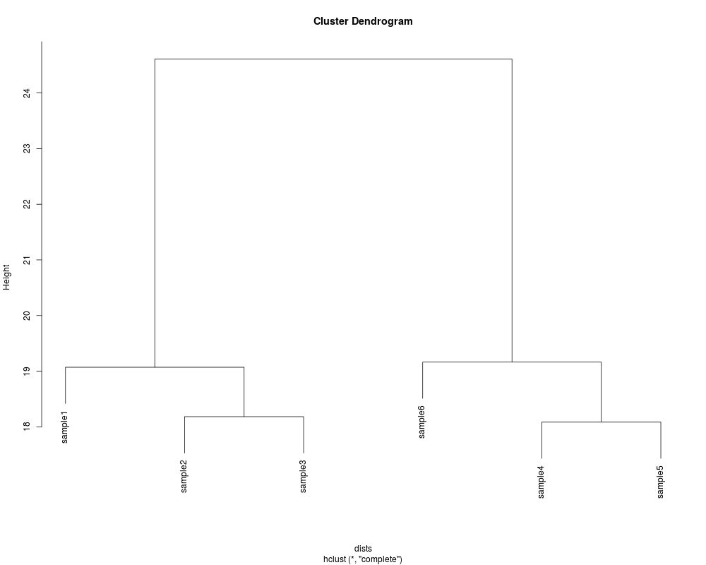
dists <- dist(t(assay(rld)))
plot(hclust(dists))

# run the rlog transformation on one dataset
design(dds) <- ~ 1
dds <- estimateSizeFactors(dds)
dds <- estimateDispersions(dds)
rld <- rlog(dds, blind=FALSE)

# apply the parameters to a new sample

ddsNew <- makeExampleDESeqDataSet(m=1)
mcols(ddsNew)$dispFit <- mcols(dds)$dispFit
betaPriorVar <- attr(rld,"betaPriorVar")
intercept <- mcols(rld)$rlogIntercept
rldNew <- rlog(ddsNew, blind=FALSE,
               intercept=intercept,
               betaPriorVar=betaPriorVar)

Results


R version 3.3.1 (2016-06-21) -- "Bug in Your Hair"
Copyright (C) 2016 The R Foundation for Statistical Computing
Platform: x86_64-pc-linux-gnu (64-bit)

R is free software and comes with ABSOLUTELY NO WARRANTY.
You are welcome to redistribute it under certain conditions.
Type 'license()' or 'licence()' for distribution details.

R is a collaborative project with many contributors.
Type 'contributors()' for more information and
'citation()' on how to cite R or R packages in publications.

Type 'demo()' for some demos, 'help()' for on-line help, or
'help.start()' for an HTML browser interface to help.
Type 'q()' to quit R.

> library(DESeq2)
Loading required package: S4Vectors
Loading required package: stats4
Loading required package: BiocGenerics
Loading required package: parallel

Attaching package: 'BiocGenerics'

The following objects are masked from 'package:parallel':

    clusterApply, clusterApplyLB, clusterCall, clusterEvalQ,
    clusterExport, clusterMap, parApply, parCapply, parLapply,
    parLapplyLB, parRapply, parSapply, parSapplyLB

The following objects are masked from 'package:stats':

    IQR, mad, xtabs

The following objects are masked from 'package:base':

    Filter, Find, Map, Position, Reduce, anyDuplicated, append,
    as.data.frame, cbind, colnames, do.call, duplicated, eval, evalq,
    get, grep, grepl, intersect, is.unsorted, lapply, lengths, mapply,
    match, mget, order, paste, pmax, pmax.int, pmin, pmin.int, rank,
    rbind, rownames, sapply, setdiff, sort, table, tapply, union,
    unique, unsplit


Attaching package: 'S4Vectors'

The following objects are masked from 'package:base':

    colMeans, colSums, expand.grid, rowMeans, rowSums

Loading required package: IRanges
Loading required package: GenomicRanges
Loading required package: GenomeInfoDb
Loading required package: SummarizedExperiment
Loading required package: Biobase
Welcome to Bioconductor

    Vignettes contain introductory material; view with
    'browseVignettes()'. To cite Bioconductor, see
    'citation("Biobase")', and for packages 'citation("pkgname")'.

> png(filename="/home/ddbj/snapshot/RGM3/R_BC/result/DESeq2/rlog.Rd_%03d_medium.png", width=480, height=480)
> ### Name: rlog
> ### Title: Apply a 'regularized log' transformation
> ### Aliases: rlog rlogTransformation
> 
> ### ** Examples
> 
> 
> dds <- makeExampleDESeqDataSet(m=6,betaSD=1)
> rld <- rlog(dds)
> dists <- dist(t(assay(rld)))
> plot(hclust(dists))
> 
> # run the rlog transformation on one dataset
> design(dds) <- ~ 1
> dds <- estimateSizeFactors(dds)
> dds <- estimateDispersions(dds)
gene-wise dispersion estimates
mean-dispersion relationship
final dispersion estimates
> rld <- rlog(dds, blind=FALSE)
> 
> # apply the parameters to a new sample
> 
> ddsNew <- makeExampleDESeqDataSet(m=1)
Warning message:
In DESeqDataSet(se, design = design, ignoreRank) :
  all genes have equal values for all samples. will not be able to perform differential analysis
> mcols(ddsNew)$dispFit <- mcols(dds)$dispFit
> betaPriorVar <- attr(rld,"betaPriorVar")
> intercept <- mcols(rld)$rlogIntercept
> rldNew <- rlog(ddsNew, blind=FALSE,
+                intercept=intercept,
+                betaPriorVar=betaPriorVar)
>                            
> 
> 
> 
> 
> 
> 
> dev.off()
null device 
          1 
>