Designs based on Strauss process

Description

Space-Filling Designs based on Strauss process

Usage

straussDesign(n,dimension,RND,alpha=0.5,repulsion=0.001,NMC=1000,
    constraints1D=0,repulsion1D=0.0001,seed=NULL)

Arguments

Details

Strauss designs are Space-Filling designs initially defined from Strauss process:

π (X) = k gamma^s(X)

where s(X) is is the number of pairs of points (xi,xj) of the design X = ( x1, ..., xn ight) that are separated by a distance no greater than the radius of interaction RND, k is the normalizing constant and gamma is the repulsion parameter. This distribution corresponds to the particular case alpha=0.

For the general case, a stochastic simulation is used to construct a Markov chain which converges to a spatial density of points π(X) described by the Strauss-Gibbs potential. In practice, the Metropolis-Hastings algorithm is implemented to simulate a distribution of points which converges to the stationary law:

π(X) = k exp(-U(X))

with a potentiel U defined by:

beta Sum_{i<j} phi(|| xi-xj ||)

where beta = -ln(gamma), phi (h) = (1-h/RND)^{alpha} if h <= RND and 0 otherwise.

The input parameters of straussDesign function can be interpreted as follows:

- RND is used to compute the number of pairs of points of the design separated by a distance no more than RND. A point is said "in interaction" with another if the spheres of radius RND/2 centered on these points intersect.

- alpha is the potential power alpha. The case alpha=0 corresponds to Strauss process (0-1 potential).

- repulsion is equal to the gamma parameter of the Strauss process. Note that gamma belongs to ]0,1].

- constraints1D allows to specify some constraints into the margin. If constraints1D==1, two repulsion parameters are needed: one for the all space (repulsion) and the other for the 1D projection (repulsion1D). Default values are repulsion=0.001 and repulsion1D=0.001. Note that the value of the radius of interaction in the one-dimensional axis is not an input parameter and is automatically fixed at 0.75/n.

Value

A list containing:

Author(s)

J. Franco

References

J. Franco, X. Bay, B. Corre and D. Dupuy (2008) Planification d experiences numeriques a partir du processus ponctuel de Strauss http://hal.archives-ouvertes.fr/hal-00260701/fr/ (March 06,2008).

Examples

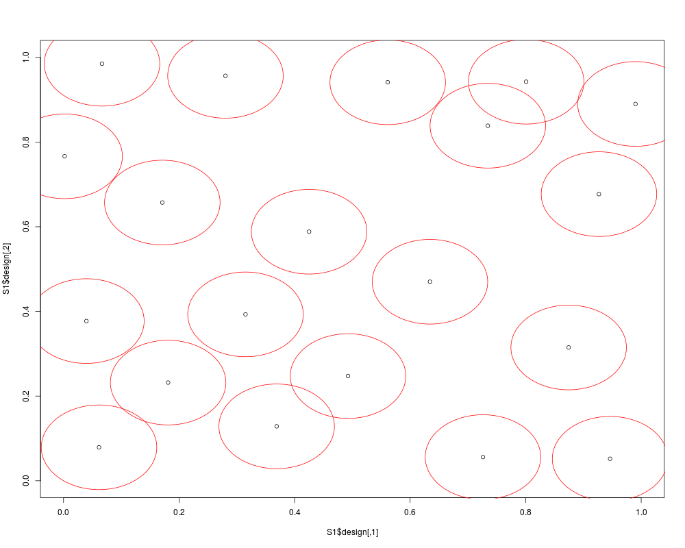
# Strauss-Gibbs designs in dimension 2 (n=20 points)
S1 <- straussDesign(n=20,dimension=2,RND=0.2)
plot(S1$design,xlim=c(0,1),ylim=c(0,1))
theta <- seq(0,2*pi,by =2*pi/(100 - 1))
for(i in 1:S1$n){
   lines(S1$design[i,1]+S1$radius/2*cos(theta),
	   S1$design[i,2]+S1$radius/2*sin(theta),col='red')
}
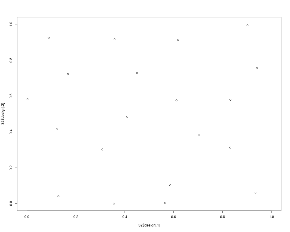
# 2D-Strauss design
S2 <- straussDesign(n=20,dimension=2,RND=0.2,NMC=200,
	constraints1D=0,alpha=0,repulsion=0.01)

plot(S2$design,xlim=c(0,1),ylim=c(0,1))

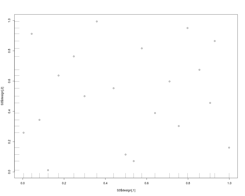
# 2D-Strauss designs with constraints on the axis
S3 <- straussDesign(n=20,dimension=2,RND=0.18,NMC=200,
	constraints1D=1,alpha=0.5,repulsion=0.1,repulsion1D=0.01)

plot(S3$design,xlim=c(0,1),ylim=c(0,1))
rug(S3$design[,1],side=1)
rug(S3$design[,2],side=2)

Results

R version 3.3.1 (2016-06-21) -- "Bug in Your Hair"
Copyright (C) 2016 The R Foundation for Statistical Computing
Platform: x86_64-pc-linux-gnu (64-bit)

R is free software and comes with ABSOLUTELY NO WARRANTY.
You are welcome to redistribute it under certain conditions.
Type 'license()' or 'licence()' for distribution details.

R is a collaborative project with many contributors.
Type 'contributors()' for more information and
'citation()' on how to cite R or R packages in publications.

Type 'demo()' for some demos, 'help()' for on-line help, or
'help.start()' for an HTML browser interface to help.
Type 'q()' to quit R.

> library(DiceDesign)
> png(filename="/home/ddbj/snapshot/RGM3/R_CC/result/DiceDesign/straussDesign.Rd_%03d_medium.png", width=480, height=480)
> ### Name: straussDesign
> ### Title: Designs based on Strauss process
> ### Aliases: straussDesign
> ### Keywords: design
> 
> ### ** Examples
> 
> # Strauss-Gibbs designs in dimension 2 (n=20 points)
> S1 <- straussDesign(n=20,dimension=2,RND=0.2)
> plot(S1$design,xlim=c(0,1),ylim=c(0,1))
> theta <- seq(0,2*pi,by =2*pi/(100 - 1))
> for(i in 1:S1$n){
+    lines(S1$design[i,1]+S1$radius/2*cos(theta),
+ 	   S1$design[i,2]+S1$radius/2*sin(theta),col='red')
+ }
> # 2D-Strauss design
> S2 <- straussDesign(n=20,dimension=2,RND=0.2,NMC=200,
+ 	constraints1D=0,alpha=0,repulsion=0.01)
> 
> plot(S2$design,xlim=c(0,1),ylim=c(0,1))
> 
> # 2D-Strauss designs with constraints on the axis
> S3 <- straussDesign(n=20,dimension=2,RND=0.18,NMC=200,
+ 	constraints1D=1,alpha=0.5,repulsion=0.1,repulsion1D=0.01)
> 
> plot(S3$design,xlim=c(0,1),ylim=c(0,1))
> rug(S3$design[,1],side=1)
> rug(S3$design[,2],side=2)
> 
> 
> 
> 
> 
> dev.off()
null device 
          1 
>