Supported by Dr. Osamu Ogasawara and  . . |
|
Last data update: 2014.03.03 |
Fit and/or create kriging modelsDescription
Usagekm(formula=~1, design, response, covtype="matern5_2", coef.trend = NULL, coef.cov = NULL, coef.var = NULL, nugget = NULL, nugget.estim=FALSE, noise.var=NULL, estim.method="MLE", penalty = NULL, optim.method = "BFGS", lower = NULL, upper = NULL, parinit = NULL, multistart = 1, control = NULL, gr = TRUE, iso=FALSE, scaling=FALSE, knots=NULL, kernel=NULL) Arguments
DetailsThe optimisers are tunable by the user by the argument
Notice that the right places to specify the optional starting values and boundaries are in
ValueAn object of class Author(s)O. Roustant, D. Ginsbourger, Ecole des Mines de St-Etienne. ReferencesN.A.C. Cressie (1993), Statistics for spatial data, Wiley series in probability and mathematical statistics. D. Ginsbourger (2009), Multiples metamodeles pour l'approximation et l'optimisation de fonctions numeriques multivariables, Ph.D. thesis, Ecole Nationale Superieure des Mines de Saint-Etienne, 2009. D. Ginsbourger, D. Dupuy, A. Badea, O. Roustant, and L. Carraro (2009), A note on the choice and the estimation of kriging models for the analysis of deterministic computer experiments, Applied Stochastic Models for Business and Industry, 25 no. 2, 115-131. A.G. Journel and M.E. Rossi (1989), When do we need a trend model in kriging ?, Mathematical Geology, 21 no. 7, 715-739. D.G. Krige (1951), A statistical approach to some basic mine valuation problems on the witwatersrand, J. of the Chem., Metal. and Mining Soc. of South Africa, 52 no. 6, 119-139. R. Li and A. Sudjianto (2005), Analysis of Computer Experiments Using Penalized Likelihood in Gaussian Kriging Models, Technometrics, 47 no. 2, 111-120. K.V. Mardia and R.J. Marshall (1984), Maximum likelihood estimation of models for residual covariance in spatial regression, Biometrika, 71, 135-146. J.D. Martin and T.W. Simpson (2005), Use of kriging models to approximate deterministic computer models, AIAA Journal, 43 no. 4, 853-863. G. Matheron (1969), Le krigeage universel, Les Cahiers du Centre de Morphologie Mathematique de Fontainebleau, 1. W.R. Jr. Mebane and J.S. Sekhon, in press (2009), Genetic optimization using derivatives: The rgenoud package for R, Journal of Statistical Software. J.-S. Park and J. Baek (2001), Efficient computation of maximum likelihood estimators in a spatial linear model with power exponential covariogram, Computer Geosciences, 27 no. 1, 1-7. C.E. Rasmussen and C.K.I. Williams (2006), Gaussian Processes for Machine Learning, the MIT Press, http://www.GaussianProcess.org/gpml See Also
Examples
# ----------------------------------
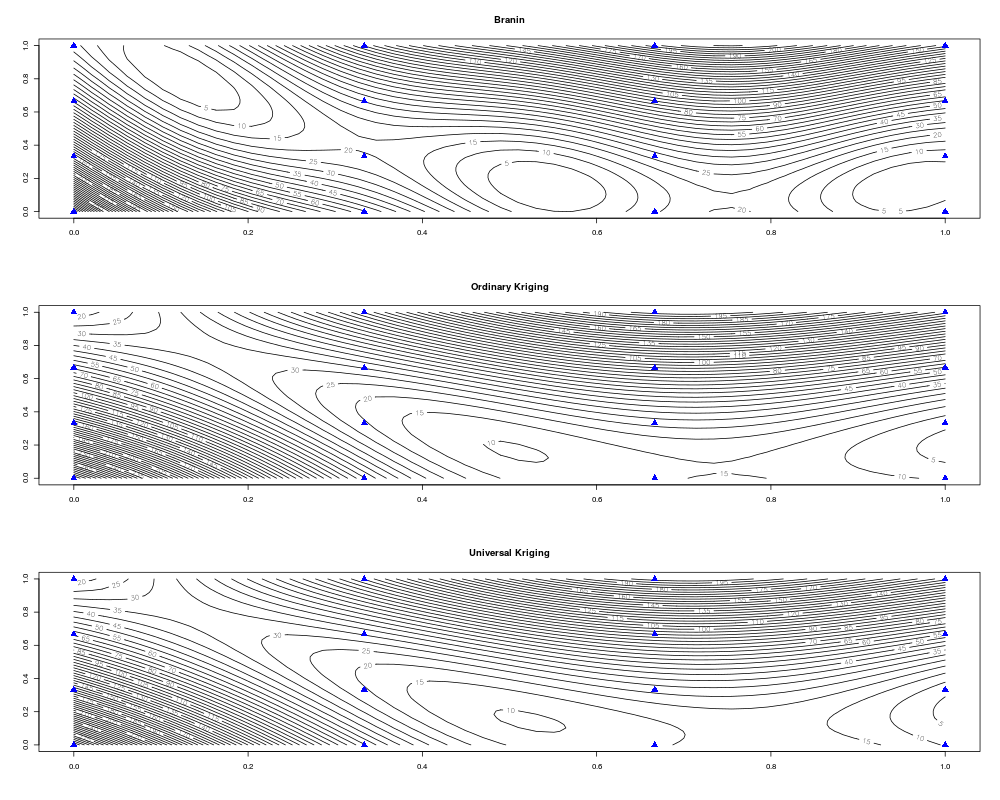
# A 2D example - Branin-Hoo function
# ----------------------------------
# a 16-points factorial design, and the corresponding response
d <- 2; n <- 16
design.fact <- expand.grid(x1=seq(0,1,length=4), x2=seq(0,1,length=4))
y <- apply(design.fact, 1, branin)
# kriging model 1 : matern5_2 covariance structure, no trend, no nugget effect
m1 <- km(design=design.fact, response=y)
# kriging model 2 : matern5_2 covariance structure,
# linear trend + interactions, no nugget effect
m2 <- km(~.^2, design=design.fact, response=y)
# graphics
n.grid <- 50
x.grid <- y.grid <- seq(0,1,length=n.grid)
design.grid <- expand.grid(x1=x.grid, x2=y.grid)
response.grid <- apply(design.grid, 1, branin)
predicted.values.model1 <- predict(m1, design.grid, "UK")$mean
predicted.values.model2 <- predict(m2, design.grid, "UK")$mean
par(mfrow=c(3,1))
contour(x.grid, y.grid, matrix(response.grid, n.grid, n.grid), 50, main="Branin")
points(design.fact[,1], design.fact[,2], pch=17, cex=1.5, col="blue")
contour(x.grid, y.grid, matrix(predicted.values.model1, n.grid, n.grid), 50,
main="Ordinary Kriging")
points(design.fact[,1], design.fact[,2], pch=17, cex=1.5, col="blue")
contour(x.grid, y.grid, matrix(predicted.values.model2, n.grid, n.grid), 50,
main="Universal Kriging")
points(design.fact[,1], design.fact[,2], pch=17, cex=1.5, col="blue")
par(mfrow=c(1,1))
# (same example) how to use the multistart argument
# -------------------------------------------------
require(foreach)
# below an example for a computer with 2 cores, but also work with 1 core
nCores <- 2
require(doParallel)
cl <- makeCluster(nCores)
registerDoParallel(cl)
# kriging model 1, with 4 starting points
m1_4 <- km(design=design.fact, response=y, multistart=4)
stopCluster(cl)
# -------------------------------
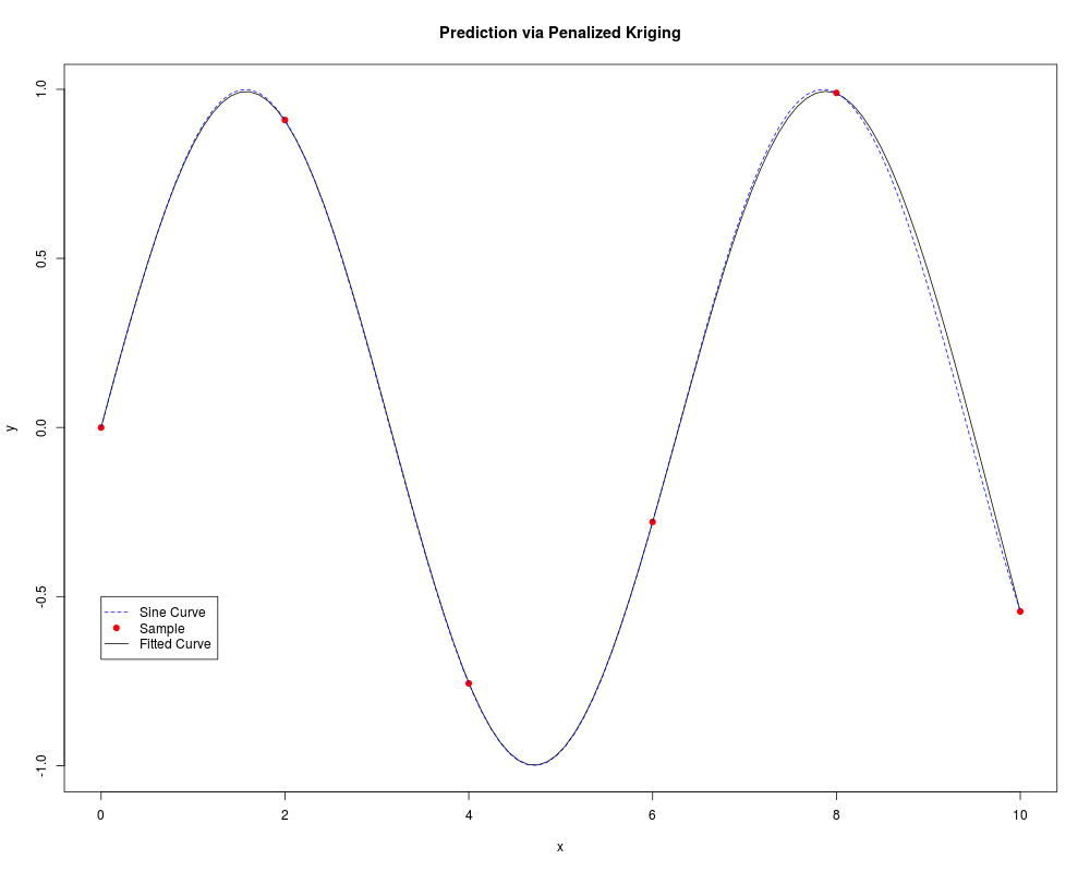
# A 1D example with penalized MLE
# -------------------------------
# from Fang K.-T., Li R. and Sudjianto A. (2006), "Design and Modeling for
# Computer Experiments", Chapman & Hall, pages 145-152
n <- 6; d <- 1
x <- seq(from=0, to=10, length=n)
y <- sin(x)
t <- seq(0,10, length=100)
# one should add a small nugget effect, to avoid numerical problems
epsilon <- 1e-3
model <- km(formula<- ~1, design=data.frame(x=x), response=data.frame(y=y),
covtype="gauss", penalty=list(fun="SCAD", value=3), nugget=epsilon)
p <- predict(model, data.frame(x=t), "UK")
plot(t, p$mean, type="l", xlab="x", ylab="y",
main="Prediction via Penalized Kriging")
points(x, y, col="red", pch=19)
lines(t, sin(t), lty=2, col="blue")
legend(0, -0.5, legend=c("Sine Curve", "Sample", "Fitted Curve"),
pch=c(-1,19,-1), lty=c(2,-1,1), col=c("blue","red","black"))
# ------------------------------------------------------------------------
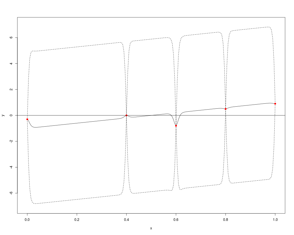
# A 1D example with known trend and known or unknown covariance parameters
# ------------------------------------------------------------------------
x <- c(0, 0.4, 0.6, 0.8, 1);
y <- c(-0.3, 0, -0.8, 0.5, 0.9)
theta <- 0.01; sigma <- 3; trend <- c(-1,2)
model <- km(~x, design=data.frame(x=x), response=data.frame(y=y),
covtype="matern5_2", coef.trend=trend, coef.cov=theta,
coef.var=sigma^2)
# below: if you want to specify trend only, and estimate both theta and sigma:
# model <- km(~x, design=data.frame(x=x), response=data.frame(y=y),
# covtype="matern5_2", coef.trend=trend, lower=0.2)
# Remark: a lower bound or penalty function is useful here,
# due to the very small number of design points...
# kriging with gaussian covariance C(x,y)=sigma^2 * exp(-[(x-y)/theta]^2),
# and linear trend t(x) = -1 + 2x
t <- seq(from=0, to=1, by=0.005)
p <- predict(model, newdata=data.frame(x=t), type="SK")
# beware that type = "SK" for known parameters (default is "UK")
plot(t, p$mean, type="l", ylim=c(-7,7), xlab="x", ylab="y")
lines(t, p$lower95, col="black", lty=2)
lines(t, p$upper95, col="black", lty=2)
points(x, y, col="red", pch=19)
abline(h=0)
# --------------------------------------------------------------
# Kriging with noisy observations (heterogeneous noise variance)
# --------------------------------------------------------------
fundet <- function(x){
return((sin(10*x)/(1+x)+2*cos(5*x)*x^3+0.841)/1.6)
}
level <- 0.5; epsilon <- 0.1
theta <- 1/sqrt(30); p <- 2; n <- 10
x <- seq(0,1, length=n)
# Heteregeneous noise variances: number of Monte Carlo evaluation among
# a total budget of 1000 stochastic simulations
MC_numbers <- c(10,50,50,290,25,75,300,10,40,150)
noise.var <- 3/MC_numbers
# Making noisy observations from 'fundet' function (defined above)
y <- fundet(x) + noise.var*rnorm(length(x))
# kriging model definition (no estimation here)
model <- km(y~1, design=data.frame(x=x), response=data.frame(y=y),
covtype="gauss", coef.trend=0, coef.cov=theta, coef.var=1,
noise.var=noise.var)
# prediction
t <- seq(0, 1, by=0.01)
p <- predict.km(model, newdata=data.frame(x=t), type="SK")
lower <- p$lower95; upper <- p$upper95
# graphics
par(mfrow=c(1,1))
plot(t, p$mean, type="l", ylim=c(1.1*min(c(lower,y)) , 1.1*max(c(upper,y))),
xlab="x", ylab="y",col="blue", lwd=1.5)
polygon(c(t,rev(t)), c(lower, rev(upper)), col=gray(0.9), border = gray(0.9))
lines(t, p$mean, type="l", ylim=c(min(lower) ,max(upper)), xlab="x", ylab="y",
col="blue", lwd=1)
lines(t, lower, col="blue", lty=4, lwd=1.7)
lines(t, upper, col="blue", lty=4, lwd=1.7)
lines(t, fundet(t), col="black", lwd=2)
points(x, y, pch=8,col="blue")
text(x, y, labels=MC_numbers, pos=3)
# -----------------------------
# Checking parameter estimation
# -----------------------------
d <- 3 # problem dimension
n <- 40 # size of the experimental design
design <- matrix(runif(n*d), n, d)
covtype <- "matern5_2"
theta <- c(0.3, 0.5, 1) # the parameters to be found by estimation
sigma <- 2
nugget <- NULL # choose a numeric value if you want to estimate nugget
nugget.estim <- FALSE # choose TRUE if you want to estimate it
n.simu <- 30 # number of simulations
sigma2.estimate <- nugget.estimate <- mu.estimate <- matrix(0, n.simu, 1)
coef.estimate <- matrix(0, n.simu, length(theta))
model <- km(~1, design=data.frame(design), response=rep(0,n), covtype=covtype,
coef.trend=0, coef.cov=theta, coef.var=sigma^2, nugget=nugget)
y <- simulate(model, nsim=n.simu)
for (i in 1:n.simu) {
# parameter estimation: tune the optimizer by changing optim.method, control
model.estimate <- km(~1, design=data.frame(design), response=data.frame(y=y[i,]),
covtype=covtype, optim.method="BFGS", control=list(pop.size=50, trace=FALSE),
nugget.estim=nugget.estim)
# store results
coef.estimate[i,] <- covparam2vect(model.estimate@covariance)
sigma2.estimate[i] <- model.estimate@covariance@sd2
mu.estimate[i] <- model.estimate@trend.coef
if (nugget.estim) nugget.estimate[i] <- model.estimate@covariance@nugget
}
# comparison true values / estimation
cat("\nResults with ", n, "design points,
obtained with ", n.simu, "simulations\n\n",
"Median of covar. coef. estimates: ", apply(coef.estimate, 2, median), "\n",
"Median of trend coef. estimates: ", median(mu.estimate), "\n",
"Mean of the var. coef. estimates: ", mean(sigma2.estimate))
if (nugget.estim) cat("\nMean of the nugget effect estimates: ",
mean(nugget.estimate))
# one figure for this specific example - to be adapted
split.screen(c(2,1)) # split display into two screens
split.screen(c(1,2), screen = 2) # now split the bottom half into 3
screen(1)
boxplot(coef.estimate[,1], coef.estimate[,2], coef.estimate[,3],
names=c("theta1", "theta2", "theta3"))
abline(h=theta, col="red")
fig.title <- paste("Empirical law of the parameter estimates
(n=", n , ", n.simu=", n.simu, ")", sep="")
title(fig.title)
screen(3)
boxplot(mu.estimate, xlab="mu")
abline(h=0, col="red")
screen(4)
boxplot(sigma2.estimate, xlab="sigma2")
abline(h=sigma^2, col="red")
close.screen(all = TRUE)
# ----------------------------------------------------------
# Kriging with non-linear scaling on Xiong et al.'s function
# ----------------------------------------------------------
f11_xiong <- function(x){
return( sin(30*(x - 0.9)^4)*cos(2*(x - 0.9)) + (x - 0.9)/2)
}
t <- seq(0,1,,300)
f <- f11_xiong(t)
plot(t,f,type="l", ylim=c(-1,0.6), lwd=2)
doe <- data.frame(x=seq(0,1,,20))
resp <- f11_xiong(doe)
knots <- list( c(0,0.5,1) )
eta <- list(c(15, 2, 0.5))
m <- km(design=doe, response=resp, scaling=TRUE, gr=TRUE,
knots=knots, covtype="matern5_2", coef.var=1, coef.trend=0)
p <- predict(m, data.frame(x=t), "UK")
plot(t, f, type="l", ylim=c(-1,0.6), lwd=2)
lines(t, p$mean, col="blue", lty=2, lwd=2)
lines(t, p$mean + 2*p$sd, col="blue")
lines(t, p$mean - 2*p$sd,col="blue")
abline(v=knots[[1]], lty=2, col="green")
# -----------------------------------------------------
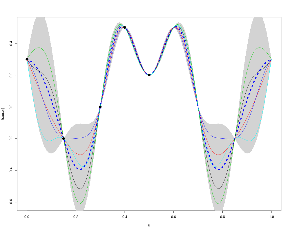
# Kriging with a symmetric kernel: example with covUser
# -----------------------------------------------------
x <- c(0, 0.15, 0.3, 0.4, 0.5)
y <- c(0.3, -0.2, 0, 0.5, 0.2)
k <- function(x,y) {
theta <- 0.15
0.5*exp(-((x-y)/theta)^2) + 0.5*exp(-((1-x-y)/theta)^2)
}
muser <- km(design=data.frame(x=x), response=data.frame(y=y),
coef.trend=0, kernel=k)
u <- seq(from=0, to=1, by=0.01)
puser <- predict(muser, newdata=data.frame(x=u), type="SK")
set.seed(0)
nsim <- 5
zuser <- simulate(muser, nsim=nsim, newdata=data.frame(x=u), cond=TRUE, nugget.sim=1e-8)
par(mfrow=c(1,1))
matplot(u, t(zuser), type="l", lty=rep("solid", nsim), col=1:5, lwd=1)
polygon(c(u, rev(u)), c(puser$upper, rev(puser$lower)), col="lightgrey", border=NA)
lines(u, puser$mean, lwd=5, col="blue", lty="dotted")
matlines(u, t(zuser), type="l", lty=rep("solid", nsim), col=1:5, lwd=1)
points(x, y, pch=19, cex=1.5)
Results
R version 3.3.1 (2016-06-21) -- "Bug in Your Hair"
Copyright (C) 2016 The R Foundation for Statistical Computing
Platform: x86_64-pc-linux-gnu (64-bit)
R is free software and comes with ABSOLUTELY NO WARRANTY.
You are welcome to redistribute it under certain conditions.
Type 'license()' or 'licence()' for distribution details.
R is a collaborative project with many contributors.
Type 'contributors()' for more information and
'citation()' on how to cite R or R packages in publications.
Type 'demo()' for some demos, 'help()' for on-line help, or
'help.start()' for an HTML browser interface to help.
Type 'q()' to quit R.
> library(DiceKriging)
> png(filename="/home/ddbj/snapshot/RGM3/R_CC/result/DiceKriging/km.Rd_%03d_medium.png", width=480, height=480)
> ### Name: km
> ### Title: Fit and/or create kriging models
> ### Aliases: km
> ### Keywords: models htest
>
> ### ** Examples
>
>
> # ----------------------------------
> # A 2D example - Branin-Hoo function
> # ----------------------------------
>
> # a 16-points factorial design, and the corresponding response
> d <- 2; n <- 16
> design.fact <- expand.grid(x1=seq(0,1,length=4), x2=seq(0,1,length=4))
> y <- apply(design.fact, 1, branin)
>
> # kriging model 1 : matern5_2 covariance structure, no trend, no nugget effect
> m1 <- km(design=design.fact, response=y)
optimisation start
------------------
* estimation method : MLE
* optimisation method : BFGS
* analytical gradient : used
* trend model : ~1
* covariance model :
- type : matern5_2
- nugget : NO
- parameters lower bounds : 1e-10 1e-10
- parameters upper bounds : 2 2
- best initial criterion value(s) : -81.26277
N = 2, M = 5 machine precision = 2.22045e-16
At X0, 0 variables are exactly at the bounds
At iterate 0 f= 81.263 |proj g|= 0.60515
At iterate 1 f = 81.236 |proj g|= 0.086174
At iterate 2 f = 81.059 |proj g|= 0.18172
At iterate 3 f = 81.058 |proj g|= 0.0018554
At iterate 4 f = 81.058 |proj g|= 3.7417e-05
iterations 4
function evaluations 6
segments explored during Cauchy searches 6
BFGS updates skipped 0
active bounds at final generalized Cauchy point 1
norm of the final projected gradient 3.7417e-05
final function value 81.0576
F = 81.0576
final value 81.057643
converged
>
> # kriging model 2 : matern5_2 covariance structure,
> # linear trend + interactions, no nugget effect
> m2 <- km(~.^2, design=design.fact, response=y)
optimisation start
------------------
* estimation method : MLE
* optimisation method : BFGS
* analytical gradient : used
* trend model : ~x1 + x2 + x1:x2
* covariance model :
- type : matern5_2
- nugget : NO
- parameters lower bounds : 1e-10 1e-10
- parameters upper bounds : 2 2
- best initial criterion value(s) : -77.70194
N = 2, M = 5 machine precision = 2.22045e-16
At X0, 0 variables are exactly at the bounds
At iterate 0 f= 77.702 |proj g|= 0.80168
At iterate 1 f = 77.691 |proj g|= 0.58884
At iterate 2 f = 77.606 |proj g|= 0.21021
At iterate 3 f = 77.545 |proj g|= 0.3489
At iterate 4 f = 77.543 |proj g|= 0.13578
At iterate 5 f = 77.543 |proj g|= 0.0036958
At iterate 6 f = 77.543 |proj g|= 4.0832e-05
At iterate 7 f = 77.543 |proj g|= 1.2468e-08
iterations 7
function evaluations 9
segments explored during Cauchy searches 9
BFGS updates skipped 0
active bounds at final generalized Cauchy point 1
norm of the final projected gradient 1.24683e-08
final function value 77.5425
F = 77.5425
final value 77.542533
converged
>
> # graphics
> n.grid <- 50
> x.grid <- y.grid <- seq(0,1,length=n.grid)
> design.grid <- expand.grid(x1=x.grid, x2=y.grid)
> response.grid <- apply(design.grid, 1, branin)
> predicted.values.model1 <- predict(m1, design.grid, "UK")$mean
> predicted.values.model2 <- predict(m2, design.grid, "UK")$mean
> par(mfrow=c(3,1))
> contour(x.grid, y.grid, matrix(response.grid, n.grid, n.grid), 50, main="Branin")
> points(design.fact[,1], design.fact[,2], pch=17, cex=1.5, col="blue")
> contour(x.grid, y.grid, matrix(predicted.values.model1, n.grid, n.grid), 50,
+ main="Ordinary Kriging")
> points(design.fact[,1], design.fact[,2], pch=17, cex=1.5, col="blue")
> contour(x.grid, y.grid, matrix(predicted.values.model2, n.grid, n.grid), 50,
+ main="Universal Kriging")
> points(design.fact[,1], design.fact[,2], pch=17, cex=1.5, col="blue")
> par(mfrow=c(1,1))
>
>
> # (same example) how to use the multistart argument
> # -------------------------------------------------
> require(foreach)
Loading required package: foreach
>
> # below an example for a computer with 2 cores, but also work with 1 core
>
> nCores <- 2
> require(doParallel)
Loading required package: doParallel
Loading required package: iterators
Loading required package: parallel
> cl <- makeCluster(nCores)
> registerDoParallel(cl)
>
> # kriging model 1, with 4 starting points
> m1_4 <- km(design=design.fact, response=y, multistart=4)
optimisation start
------------------
* estimation method : MLE
* optimisation method : BFGS
* analytical gradient : used
* trend model : ~1
* covariance model :
- type : matern5_2
- nugget : NO
- parameters lower bounds : 1e-10 1e-10
- parameters upper bounds : 2 2
- best initial criterion value(s) : -83.11173 -83.51967 -83.69294 -84.31335
* The 4 best values (multistart) obtained are:
81.05764 81.05764 81.05764 81.05764
* The model corresponding to the best one (81.05764) is stored.
>
> stopCluster(cl)
>
> # -------------------------------
> # A 1D example with penalized MLE
> # -------------------------------
>
> # from Fang K.-T., Li R. and Sudjianto A. (2006), "Design and Modeling for
> # Computer Experiments", Chapman & Hall, pages 145-152
>
> n <- 6; d <- 1
> x <- seq(from=0, to=10, length=n)
> y <- sin(x)
> t <- seq(0,10, length=100)
>
> # one should add a small nugget effect, to avoid numerical problems
> epsilon <- 1e-3
> model <- km(formula<- ~1, design=data.frame(x=x), response=data.frame(y=y),
+ covtype="gauss", penalty=list(fun="SCAD", value=3), nugget=epsilon)
optimisation start
------------------
* estimation method : PMLE
* optimisation method : BFGS
* analytical gradient : used
* trend model : ~1
* covariance model :
- type : gauss
- nugget : 0.001
- parameters lower bounds : 1e-10
- parameters upper bounds : 20
- variance bounds : 0.02920568 5.461071
- best initial criterion value(s) : -14.62764
N = 2, M = 5 machine precision = 2.22045e-16
At X0, 0 variables are exactly at the bounds
At iterate 0 f= 14.628 |proj g|= 4.4439
At iterate 1 f = 12.692 |proj g|= 0.7852
At iterate 2 f = 12.669 |proj g|= 0.065698
At iterate 3 f = 12.665 |proj g|= 0.059133
At iterate 4 f = 12.635 |proj g|= 0.61518
At iterate 5 f = 12.62 |proj g|= 0.51764
At iterate 6 f = 12.603 |proj g|= 0.098535
At iterate 7 f = 12.603 |proj g|= 0.040403
At iterate 8 f = 12.603 |proj g|= 0.0012506
At iterate 9 f = 12.603 |proj g|= 0.00043058
At iterate 10 f = 12.603 |proj g|= 0.00022011
iterations 10
function evaluations 12
segments explored during Cauchy searches 10
BFGS updates skipped 0
active bounds at final generalized Cauchy point 0
norm of the final projected gradient 0.00022011
final function value 12.6026
F = 12.6026
final value 12.602552
converged
>
> p <- predict(model, data.frame(x=t), "UK")
>
> plot(t, p$mean, type="l", xlab="x", ylab="y",
+ main="Prediction via Penalized Kriging")
> points(x, y, col="red", pch=19)
> lines(t, sin(t), lty=2, col="blue")
> legend(0, -0.5, legend=c("Sine Curve", "Sample", "Fitted Curve"),
+ pch=c(-1,19,-1), lty=c(2,-1,1), col=c("blue","red","black"))
>
>
> # ------------------------------------------------------------------------
> # A 1D example with known trend and known or unknown covariance parameters
> # ------------------------------------------------------------------------
>
> x <- c(0, 0.4, 0.6, 0.8, 1);
> y <- c(-0.3, 0, -0.8, 0.5, 0.9)
>
> theta <- 0.01; sigma <- 3; trend <- c(-1,2)
>
> model <- km(~x, design=data.frame(x=x), response=data.frame(y=y),
+ covtype="matern5_2", coef.trend=trend, coef.cov=theta,
+ coef.var=sigma^2)
>
> # below: if you want to specify trend only, and estimate both theta and sigma:
> # model <- km(~x, design=data.frame(x=x), response=data.frame(y=y),
> # covtype="matern5_2", coef.trend=trend, lower=0.2)
> # Remark: a lower bound or penalty function is useful here,
> # due to the very small number of design points...
>
> # kriging with gaussian covariance C(x,y)=sigma^2 * exp(-[(x-y)/theta]^2),
> # and linear trend t(x) = -1 + 2x
>
> t <- seq(from=0, to=1, by=0.005)
> p <- predict(model, newdata=data.frame(x=t), type="SK")
> # beware that type = "SK" for known parameters (default is "UK")
>
> plot(t, p$mean, type="l", ylim=c(-7,7), xlab="x", ylab="y")
> lines(t, p$lower95, col="black", lty=2)
> lines(t, p$upper95, col="black", lty=2)
> points(x, y, col="red", pch=19)
> abline(h=0)
>
>
> # --------------------------------------------------------------
> # Kriging with noisy observations (heterogeneous noise variance)
> # --------------------------------------------------------------
>
> fundet <- function(x){
+ return((sin(10*x)/(1+x)+2*cos(5*x)*x^3+0.841)/1.6)
+ }
>
> level <- 0.5; epsilon <- 0.1
> theta <- 1/sqrt(30); p <- 2; n <- 10
> x <- seq(0,1, length=n)
>
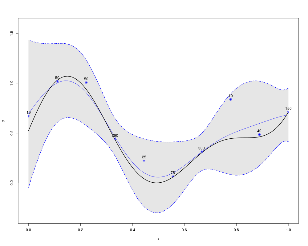
> # Heteregeneous noise variances: number of Monte Carlo evaluation among
> # a total budget of 1000 stochastic simulations
> MC_numbers <- c(10,50,50,290,25,75,300,10,40,150)
> noise.var <- 3/MC_numbers
>
> # Making noisy observations from 'fundet' function (defined above)
> y <- fundet(x) + noise.var*rnorm(length(x))
>
> # kriging model definition (no estimation here)
> model <- km(y~1, design=data.frame(x=x), response=data.frame(y=y),
+ covtype="gauss", coef.trend=0, coef.cov=theta, coef.var=1,
+ noise.var=noise.var)
>
> # prediction
> t <- seq(0, 1, by=0.01)
> p <- predict.km(model, newdata=data.frame(x=t), type="SK")
> lower <- p$lower95; upper <- p$upper95
>
> # graphics
> par(mfrow=c(1,1))
> plot(t, p$mean, type="l", ylim=c(1.1*min(c(lower,y)) , 1.1*max(c(upper,y))),
+ xlab="x", ylab="y",col="blue", lwd=1.5)
> polygon(c(t,rev(t)), c(lower, rev(upper)), col=gray(0.9), border = gray(0.9))
> lines(t, p$mean, type="l", ylim=c(min(lower) ,max(upper)), xlab="x", ylab="y",
+ col="blue", lwd=1)
> lines(t, lower, col="blue", lty=4, lwd=1.7)
> lines(t, upper, col="blue", lty=4, lwd=1.7)
> lines(t, fundet(t), col="black", lwd=2)
> points(x, y, pch=8,col="blue")
> text(x, y, labels=MC_numbers, pos=3)
>
>
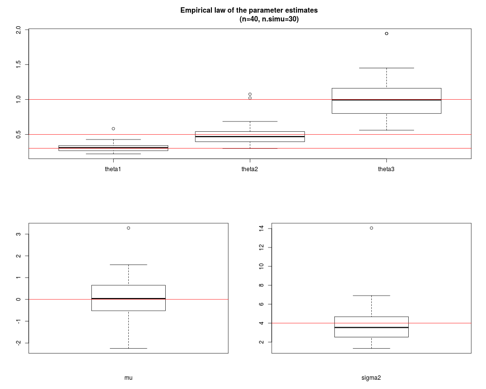
> # -----------------------------
> # Checking parameter estimation
> # -----------------------------
>
> d <- 3 # problem dimension
> n <- 40 # size of the experimental design
> design <- matrix(runif(n*d), n, d)
>
> covtype <- "matern5_2"
> theta <- c(0.3, 0.5, 1) # the parameters to be found by estimation
> sigma <- 2
> nugget <- NULL # choose a numeric value if you want to estimate nugget
> nugget.estim <- FALSE # choose TRUE if you want to estimate it
>
> n.simu <- 30 # number of simulations
> sigma2.estimate <- nugget.estimate <- mu.estimate <- matrix(0, n.simu, 1)
> coef.estimate <- matrix(0, n.simu, length(theta))
>
> model <- km(~1, design=data.frame(design), response=rep(0,n), covtype=covtype,
+ coef.trend=0, coef.cov=theta, coef.var=sigma^2, nugget=nugget)
> y <- simulate(model, nsim=n.simu)
>
> for (i in 1:n.simu) {
+ # parameter estimation: tune the optimizer by changing optim.method, control
+ model.estimate <- km(~1, design=data.frame(design), response=data.frame(y=y[i,]),
+ covtype=covtype, optim.method="BFGS", control=list(pop.size=50, trace=FALSE),
+ nugget.estim=nugget.estim)
+
+ # store results
+ coef.estimate[i,] <- covparam2vect(model.estimate@covariance)
+ sigma2.estimate[i] <- model.estimate@covariance@sd2
+ mu.estimate[i] <- model.estimate@trend.coef
+ if (nugget.estim) nugget.estimate[i] <- model.estimate@covariance@nugget
+ }
>
> # comparison true values / estimation
> cat("\nResults with ", n, "design points,
+ obtained with ", n.simu, "simulations\n\n",
+ "Median of covar. coef. estimates: ", apply(coef.estimate, 2, median), "\n",
+ "Median of trend coef. estimates: ", median(mu.estimate), "\n",
+ "Mean of the var. coef. estimates: ", mean(sigma2.estimate))
Results with 40 design points,
obtained with 30 simulations
Median of covar. coef. estimates: 0.2962495 0.5876976 1.028413
Median of trend coef. estimates: 0.3880651
Mean of the var. coef. estimates: 4.185776> if (nugget.estim) cat("\nMean of the nugget effect estimates: ",
+ mean(nugget.estimate))
>
> # one figure for this specific example - to be adapted
> split.screen(c(2,1)) # split display into two screens
[1] 1 2
> split.screen(c(1,2), screen = 2) # now split the bottom half into 3
[1] 3 4
>
> screen(1)
> boxplot(coef.estimate[,1], coef.estimate[,2], coef.estimate[,3],
+ names=c("theta1", "theta2", "theta3"))
> abline(h=theta, col="red")
> fig.title <- paste("Empirical law of the parameter estimates
+ (n=", n , ", n.simu=", n.simu, ")", sep="")
> title(fig.title)
>
> screen(3)
> boxplot(mu.estimate, xlab="mu")
> abline(h=0, col="red")
>
> screen(4)
> boxplot(sigma2.estimate, xlab="sigma2")
> abline(h=sigma^2, col="red")
>
> close.screen(all = TRUE)
>
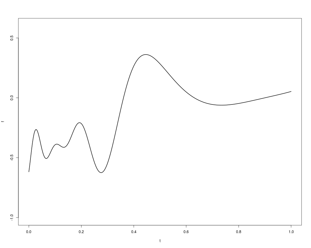
> # ----------------------------------------------------------
> # Kriging with non-linear scaling on Xiong et al.'s function
> # ----------------------------------------------------------
>
> f11_xiong <- function(x){
+ return( sin(30*(x - 0.9)^4)*cos(2*(x - 0.9)) + (x - 0.9)/2)
+ }
>
> t <- seq(0,1,,300)
> f <- f11_xiong(t)
>
> plot(t,f,type="l", ylim=c(-1,0.6), lwd=2)
>
> doe <- data.frame(x=seq(0,1,,20))
> resp <- f11_xiong(doe)
>
> knots <- list( c(0,0.5,1) )
> eta <- list(c(15, 2, 0.5))
> m <- km(design=doe, response=resp, scaling=TRUE, gr=TRUE,
+ knots=knots, covtype="matern5_2", coef.var=1, coef.trend=0)
optimisation start
------------------
* estimation method : MLE
* optimisation method : BFGS
* analytical gradient : used
* trend model : ~1
* covariance model :
- type : matern5_2
- nugget : NO
- parameters lower bounds : 0.5 0.5 0.5
- parameters upper bounds : 1e+10 1e+10 1e+10
- best initial criterion value(s) : 21.32984
N = 3, M = 5 machine precision = 2.22045e-16
At X0, 0 variables are exactly at the bounds
At iterate 0 f= -21.33 |proj g|= 2.0761
At iterate 1 f = -28.162 |proj g|= 1.4412
ys=-3.141e+00 -gs= 5.425e+00, BFGS update SKIPPED
At iterate 2 f = -32.285 |proj g|= 1.27
At iterate 3 f = -32.364 |proj g|= 0.53883
At iterate 4 f = -32.436 |proj g|= 0.33819
At iterate 5 f = -32.439 |proj g|= 0.082465
At iterate 6 f = -32.441 |proj g|= 0.30521
At iterate 7 f = -32.448 |proj g|= 0.54429
At iterate 8 f = -32.473 |proj g|= 0.96092
At iterate 9 f = -32.499 |proj g|= 0.88238
At iterate 10 f = -32.508 |proj g|= 0.38697
At iterate 11 f = -32.515 |proj g|= 0.26533
At iterate 12 f = -32.517 |proj g|= 0.050816
At iterate 13 f = -32.517 |proj g|= 0.0018408
At iterate 14 f = -32.517 |proj g|= 1.7013e-05
At iterate 15 f = -32.517 |proj g|= 1.5422e-05
iterations 15
function evaluations 21
segments explored during Cauchy searches 16
BFGS updates skipped 1
active bounds at final generalized Cauchy point 0
norm of the final projected gradient 1.54216e-05
final function value -32.5166
F = -32.5166
final value -32.516606
converged
>
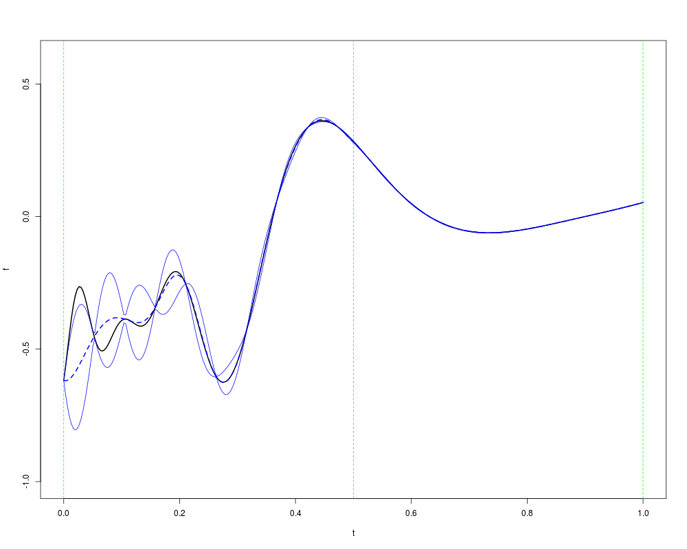
> p <- predict(m, data.frame(x=t), "UK")
>
> plot(t, f, type="l", ylim=c(-1,0.6), lwd=2)
>
> lines(t, p$mean, col="blue", lty=2, lwd=2)
> lines(t, p$mean + 2*p$sd, col="blue")
> lines(t, p$mean - 2*p$sd,col="blue")
>
> abline(v=knots[[1]], lty=2, col="green")
>
>
> # -----------------------------------------------------
> # Kriging with a symmetric kernel: example with covUser
> # -----------------------------------------------------
>
> x <- c(0, 0.15, 0.3, 0.4, 0.5)
> y <- c(0.3, -0.2, 0, 0.5, 0.2)
>
> k <- function(x,y) {
+ theta <- 0.15
+ 0.5*exp(-((x-y)/theta)^2) + 0.5*exp(-((1-x-y)/theta)^2)
+ }
>
> muser <- km(design=data.frame(x=x), response=data.frame(y=y),
+ coef.trend=0, kernel=k)
>
> u <- seq(from=0, to=1, by=0.01)
> puser <- predict(muser, newdata=data.frame(x=u), type="SK")
>
> set.seed(0)
> nsim <- 5
> zuser <- simulate(muser, nsim=nsim, newdata=data.frame(x=u), cond=TRUE, nugget.sim=1e-8)
> par(mfrow=c(1,1))
> matplot(u, t(zuser), type="l", lty=rep("solid", nsim), col=1:5, lwd=1)
> polygon(c(u, rev(u)), c(puser$upper, rev(puser$lower)), col="lightgrey", border=NA)
> lines(u, puser$mean, lwd=5, col="blue", lty="dotted")
> matlines(u, t(zuser), type="l", lty=rep("solid", nsim), col=1:5, lwd=1)
> points(x, y, pch=19, cex=1.5)
>
>
>
>
>
>
> dev.off()
null device
1
>
|