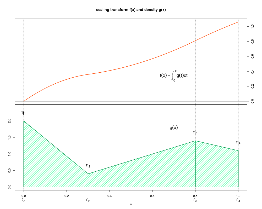
Scaling function

Description

Parametric transformation of the input space variables. The transformation is obtained coordinatewise by integrating piecewise affine marginal "densities" parametrized by a vector of knots and a matrix of density values at the knots. See references for more detail.

Usage

scalingFun(X, knots, eta, plot=FALSE)

Arguments

Value

The image of X by a scaling transformation of parameters knots and eta

References

Y. Xiong, W. Chen, D. Apley, and X. Ding (2007), Int. J. Numer. Meth. Engng, A non-stationary covariance-based Kriging method for metamodelling in engineering design.

See Also

scalingGrad

Examples

## 1D Transform of Xiong et al.
knots <- c(0, 0.3, 0.8, 1); eta <- c(2, 0.4, 1.4, 1.1)
nk <- length(knots)
t <- seq(from = 0, to = 1, length = 200)
f <- scalingFun(X = matrix(t), knots = list(knots), eta = list(eta))

## for text positions only
itext <- round(length(t) * 0.7)
xtext <- t[itext]; ftext <- f[itext] / 2; etamax <- max(eta)

## plot the transform function
opar <- par(mfrow = c(2, 1))
par(mar = c(0, 4, 5, 4))
plot(x = t, y = f, type = "l", lwd = 2, col = "orangered",
     main = "scaling transform f(x) and density g(x)",
     xlab = "", ylab = "", xaxt = "n", yaxt = "n") 
axis(side = 4)
abline(v = knots, lty = "dotted"); abline(h = 0)
text(x = xtext, y = ftext, cex = 1.4,
     labels = expression(f(x) == integral(g(t)*dt, 0, x)))

## plot the density function, which is piecewise linear
scalingDens1d <- approxfun(x = knots, y = eta)
g <- scalingDens1d(t)
gtext <- 0.5 * g[itext] + 0.6 * etamax
par(mar = c(5, 4, 0, 4))
plot(t, g, type = "l", lwd = 2, ylim = c(0, etamax * 1.2),
     col = "SpringGreen4", xlab = expression(x), ylab ="")
abline(v = knots, lty = "dotted")
lines(x = knots, y = eta, lty = 1, lwd = 2, type = "h", col = "SpringGreen4")
abline(h = 0)
text(x = 0.7, y = gtext, cex = 1.4, labels = expression(g(x)))

## show knots with math symbols eta, zeta
for (i in 1:nk) {
  text(x = knots[i], y = eta[i] + 0.12 * etamax, cex = 1.4,
       labels = substitute(eta[i], list(i = i)))
  mtext(side = 1, cex = 1.4, at = knots[i], line = 2.4,
        text = substitute(zeta[i], list(i = i)))
}
polygon(x = c(knots, knots[nk], knots[1]),  y = c(eta, 0, 0),
        density = 15, angle = 45, col = "SpringGreen", border = NA)
par(opar)

Results

R version 3.3.1 (2016-06-21) -- "Bug in Your Hair"
Copyright (C) 2016 The R Foundation for Statistical Computing
Platform: x86_64-pc-linux-gnu (64-bit)

R is free software and comes with ABSOLUTELY NO WARRANTY.
You are welcome to redistribute it under certain conditions.
Type 'license()' or 'licence()' for distribution details.

R is a collaborative project with many contributors.
Type 'contributors()' for more information and
'citation()' on how to cite R or R packages in publications.

Type 'demo()' for some demos, 'help()' for on-line help, or
'help.start()' for an HTML browser interface to help.
Type 'q()' to quit R.

> library(DiceKriging)
> png(filename="/home/ddbj/snapshot/RGM3/R_CC/result/DiceKriging/scalingFun.Rd_%03d_medium.png", width=480, height=480)
> ### Name: scalingFun
> ### Title: Scaling function
> ### Aliases: scalingFun
> ### Keywords: models
> 
> ### ** Examples
> 
> ## 1D Transform of Xiong et al.
> knots <- c(0, 0.3, 0.8, 1); eta <- c(2, 0.4, 1.4, 1.1)
> nk <- length(knots)
> t <- seq(from = 0, to = 1, length = 200)
> f <- scalingFun(X = matrix(t), knots = list(knots), eta = list(eta))
> 
> ## for text positions only
> itext <- round(length(t) * 0.7)
> xtext <- t[itext]; ftext <- f[itext] / 2; etamax <- max(eta)
> 
> ## plot the transform function
> opar <- par(mfrow = c(2, 1))
> par(mar = c(0, 4, 5, 4))
> plot(x = t, y = f, type = "l", lwd = 2, col = "orangered",
+      main = "scaling transform f(x) and density g(x)",
+      xlab = "", ylab = "", xaxt = "n", yaxt = "n") 
> axis(side = 4)
> abline(v = knots, lty = "dotted"); abline(h = 0)
> text(x = xtext, y = ftext, cex = 1.4,
+      labels = expression(f(x) == integral(g(t)*dt, 0, x)))
> 
> ## plot the density function, which is piecewise linear
> scalingDens1d <- approxfun(x = knots, y = eta)
> g <- scalingDens1d(t)
> gtext <- 0.5 * g[itext] + 0.6 * etamax
> par(mar = c(5, 4, 0, 4))
> plot(t, g, type = "l", lwd = 2, ylim = c(0, etamax * 1.2),
+      col = "SpringGreen4", xlab = expression(x), ylab ="")
> abline(v = knots, lty = "dotted")
> lines(x = knots, y = eta, lty = 1, lwd = 2, type = "h", col = "SpringGreen4")
> abline(h = 0)
> text(x = 0.7, y = gtext, cex = 1.4, labels = expression(g(x)))
> 
> ## show knots with math symbols eta, zeta
> for (i in 1:nk) {
+   text(x = knots[i], y = eta[i] + 0.12 * etamax, cex = 1.4,
+        labels = substitute(eta[i], list(i = i)))
+   mtext(side = 1, cex = 1.4, at = knots[i], line = 2.4,
+         text = substitute(zeta[i], list(i = i)))
+ }
> polygon(x = c(knots, knots[nk], knots[1]),  y = c(eta, 0, 0),
+         density = 15, angle = 45, col = "SpringGreen", border = NA)
> par(opar)
> 
> 
> 
> 
> 
> dev.off()
null device 
          1 
>