R Graphical Manual

Browse All

Last data update: 2014.03.03

R: Simulate GP values at any given set of points for a km object

simulate

R Documentation

Simulate GP values at any given set of points for a km object

Description

simulate is used to simulate Gaussian process values at any given set of points for a specified km object.

Usage

## S4 method for signature 'km'
simulate(object, nsim=1, seed=NULL, newdata=NULL, 
                            cond=FALSE, nugget.sim=0, checkNames=TRUE, ...)

Arguments

`object`	an object of class `km`.
`nsim`	an optional number specifying the number of response vectors to simulate. Default is 1.
`seed`	usual `seed` argument of method simulate. Not used yet in `simulated.km`.
`newdata`	an optional vector, matrix or data frame containing the points where to perform predictions. Default is NULL: simulation is performed at design points specified in `object`.
`cond`	an optional boolean indicating the type of simulations. If `TRUE`, the simulations are performed conditionally to the response vector defined by using `km`, and contained in `model` (slot y: `model@y`). If `FALSE`, the simulations are non conditional. Default is `FALSE`.
`nugget.sim`	an optional number corresponding to a numerical nugget effect, which may be useful in presence of numerical instabilities. If specified, it is added to the diagonal terms of the covariance matrix (that is: `newdata` if `cond=TRUE`, or of `(newdata, model@y)` either) to ensure that it is positive definite. In any case, this parameter does not modify `model`. It has no effect if `newdata=NULL`. Default is 0.
`checkNames`	an optional boolean. If `TRUE` (default), a consistency test is performed between the names of `newdata` and the names of the experimental design (contained in `object@X`), see section Warning below.
`...`	no other argument for this method.

Value

A matrix containing the simulated response vectors at the newdata points, with one sample in each row.

Warning

The columns of newdata should correspond to the input variables, and only the input variables (nor the response is not admitted, neither external variables). If newdata contains variable names, and if checkNames is TRUE (default), then checkNames performs a complete consistency test with the names of the experimental design. Otherwise, it is assumed that its columns correspond to the same variables than the experimental design and in the same order.

Note

	1. When constructing a `km` object with known parameters, note that the argument `y` (the output) is required in `km` even if it will not be used for simulation.
	2. Sometimes, a small nugget effect is necessary to avoid numerical instabilities (see the ex. below).

Author(s)

O. Roustant, D. Ginsbourger, Ecole des Mines de St-Etienne.

References

N.A.C. Cressie (1993), Statistics for spatial data, Wiley series in probability and mathematical statistics.

A.G. Journel and C.J. Huijbregts (1978), Mining Geostatistics, Academic Press, London.

B.D. Ripley (1987), Stochastic Simulation, Wiley.

Examples



# ----------------
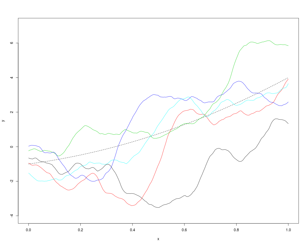
# some simulations 
# ----------------

n <- 200
x <- seq(from=0, to=1, length=n)

covtype <- "matern3_2"
coef.cov <- c(theta <- 0.3/sqrt(3))
sigma <- 1.5
trend <- c(intercept <- -1, beta1 <- 2, beta2 <- 3)
nugget <- 0   # may be sometimes a little more than zero in some cases, 
              # due to numerical instabilities

formula <- ~x+I(x^2)    # quadratic trend (beware to the usual I operator)

ytrend <- intercept + beta1*x + beta2*x^2
plot(x, ytrend, type="l", col="black", ylab="y", lty="dashed",
     ylim=c(min(ytrend)-2*sigma, max(ytrend) + 2*sigma))

model <- km(formula, design=data.frame(x=x), response=rep(0,n), 
            covtype=covtype, coef.trend=trend, coef.cov=coef.cov, 
            coef.var=sigma^2, nugget=nugget)
y <- simulate(model, nsim=5, newdata=NULL)

for (i in 1:5) {
  lines(x, y[i,], col=i)
}


# --------------------------------------------------------------------
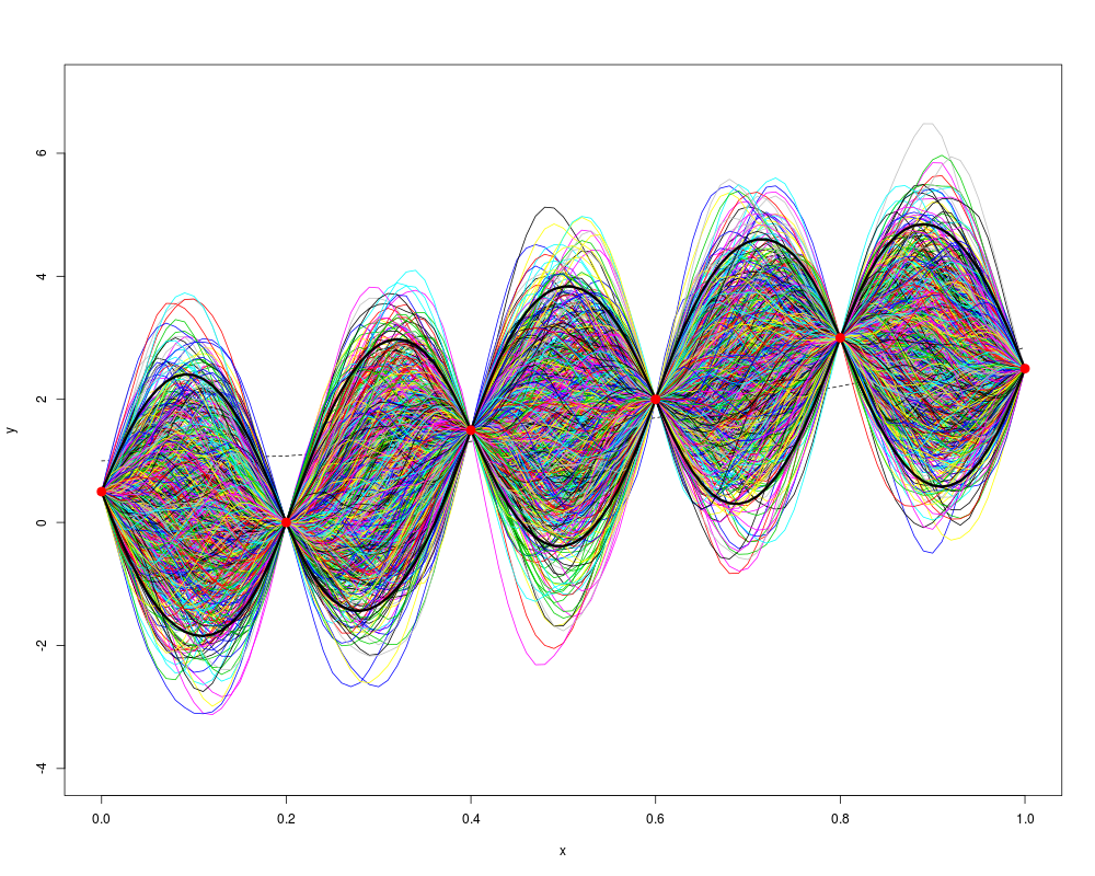
# conditional simulations and consistancy with Simple Kriging formulas
# --------------------------------------------------------------------

n <- 6
m <- 101
x <- seq(from=0, to=1, length=n)
response <- c(0.5, 0, 1.5, 2, 3, 2.5)

covtype <- "matern5_2"
coef.cov <- 0.1
sigma <- 1.5

trend <- c(intercept <- 5, beta <- -4)
model <- km(formula=~cos(x), design=data.frame(x=x), response=response, 
            covtype=covtype, coef.trend=trend, coef.cov=coef.cov, 
            coef.var=sigma^2)

t <- seq(from=0, to=1, length=m)
nsim <- 1000
y <- simulate(model, nsim=nsim, newdata=data.frame(x=t), cond=TRUE, nugget.sim=1e-5)

## graphics

plot(x, intercept + beta*cos(x), type="l", col="black", 
     ylim=c(-4, 7), ylab="y", lty="dashed")
for (i in 1:nsim) {
	lines(t, y[i,], col=i)
}

p <- predict(model, newdata=data.frame(x=t), type="SK")
lines(t, p$lower95, lwd=3)
lines(t, p$upper95, lwd=3)

points(x, response, pch=19, cex=1.5, col="red")

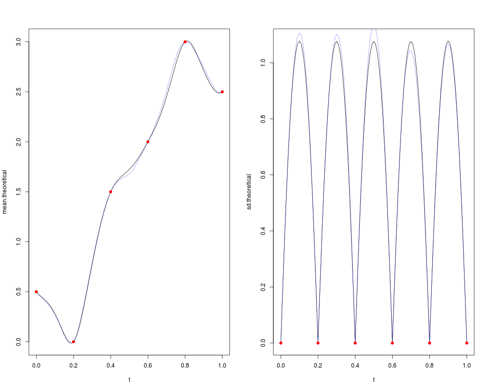
# compare theoretical kriging mean and sd with the mean and sd of
# simulated sample functions
mean.theoretical <- p$mean
sd.theoretical <- p$sd
mean.simulated <- apply(y, 2, mean) 
sd.simulated <- apply(y, 2, sd)
par(mfrow=c(1,2))
plot(t, mean.theoretical, type="l")
lines(t, mean.simulated, col="blue", lty="dotted")
points(x, response, pch=19, col="red")
plot(t, sd.theoretical, type="l")
lines(t, sd.simulated, col="blue", lty="dotted")
points(x, rep(0, n), pch=19, col="red")
par(mfrow=c(1,1))

# estimate the confidence level at each point
level <- rep(0, m)
for (j in 1:m) {
	level[j] <- sum((y[,j]>=p$lower95[j]) & (y[,j]<=p$upper95[j]))/nsim
}
level    # level computed this way may be completely wrong at interpolation 
         # points, due to the numerical errors in the calculation of the 
         # kriging mean


# ---------------------------------------------------------------------
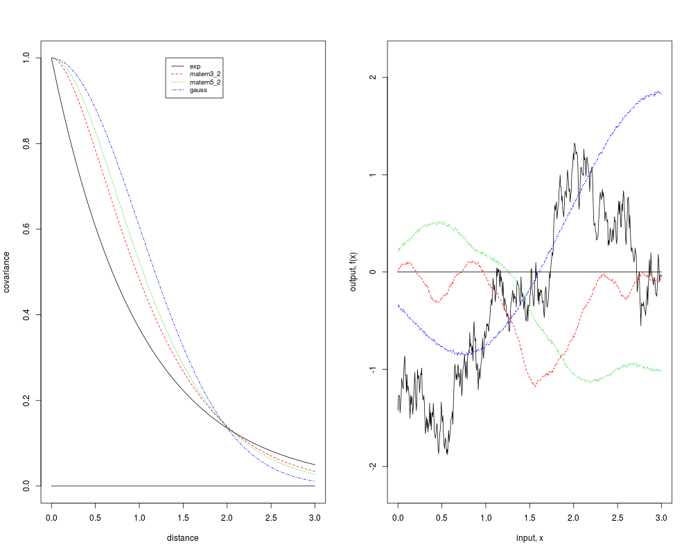
# covariance kernel + simulations for "exp", "matern 3/2", "matern 5/2" 
#                                 and "exp" covariances
# ---------------------------------------------------------------------

covtype <- c("exp", "matern3_2", "matern5_2", "gauss")

d <- 1
n <- 500
x <- seq(from=0, to=3, length=n)

par(mfrow=c(1,2))
plot(x, rep(0,n), type="l", ylim=c(0,1), xlab="distance", ylab="covariance")

param <- 1
sigma2 <- 1

for (i in 1:length(covtype)) {
	covStruct <- covStruct.create(covtype=covtype[i], d=d, known.covparam="All", 
                      var.names="x", coef.cov=param, coef.var=sigma2)
	y <- covMat1Mat2(covStruct, X1=as.matrix(x), X2=as.matrix(0))
	lines(x, y, col=i, lty=i)
	}
legend(x=1.3, y=1, legend=covtype, col=1:length(covtype), 
       lty=1:length(covtype), cex=0.8)

plot(x, rep(0,n), type="l", ylim=c(-2.2, 2.2), xlab="input, x", 
     ylab="output, f(x)")
for (i in 1:length(covtype)) {
	model <- km(~1, design=data.frame(x=x), response=rep(0,n), covtype=covtype[i], 
		    coef.trend=0, coef.cov=param, coef.var=sigma2, nugget=1e-4)
	y <- simulate(model)
	lines(x, y, col=i, lty=i)
}
par(mfrow=c(1,1))

# -------------------------------------------------------
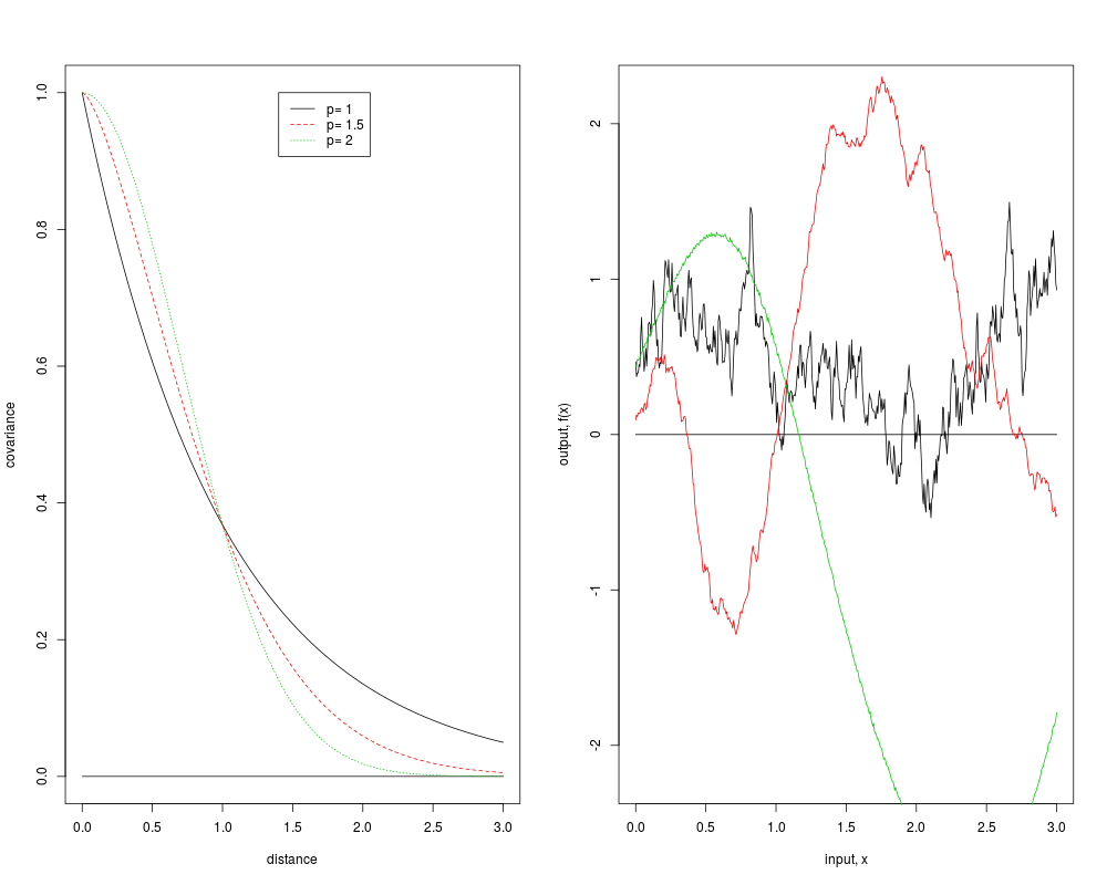
# covariance kernel + simulations for "powexp" covariance
# -------------------------------------------------------

covtype <- "powexp"

d <- 1
n <- 500
x <- seq(from=0, to=3, length=n)

par(mfrow=c(1,2))
plot(x, rep(0,n), type="l", ylim=c(0,1), xlab="distance", ylab="covariance")

param <- c(1, 1.5, 2)
sigma2 <- 1

for (i in 1:length(param)) {
	covStruct <- covStruct.create(covtype=covtype, d=d, known.covparam="All",
                      var.names="x", coef.cov=c(1, param[i]), coef.var=sigma2)
	y <- covMat1Mat2(covStruct, X1=as.matrix(x), X2=as.matrix(0))
	lines(x, y, col=i, lty=i)
	}
legend(x=1.4, y=1, legend=paste("p=", param), col=1:3, lty=1:3)

plot(x, rep(0,n), type="l", ylim=c(-2.2, 2.2), xlab="input, x", 
     ylab="output, f(x)")
for (i in 1:length(param)) {
	model <- km(~1, design=data.frame(x=x), response=rep(0,n), covtype=covtype, 
        coef.trend=0, coef.cov=c(1, param[i]), coef.var=sigma2, nugget=1e-4)
	y <- simulate(model)
	lines(x, y, col=i)
}
par(mfrow=c(1,1))

Results


R version 3.3.1 (2016-06-21) -- "Bug in Your Hair"
Copyright (C) 2016 The R Foundation for Statistical Computing
Platform: x86_64-pc-linux-gnu (64-bit)

R is free software and comes with ABSOLUTELY NO WARRANTY.
You are welcome to redistribute it under certain conditions.
Type 'license()' or 'licence()' for distribution details.

R is a collaborative project with many contributors.
Type 'contributors()' for more information and
'citation()' on how to cite R or R packages in publications.

Type 'demo()' for some demos, 'help()' for on-line help, or
'help.start()' for an HTML browser interface to help.
Type 'q()' to quit R.

> library(DiceKriging)
> png(filename="/home/ddbj/snapshot/RGM3/R_CC/result/DiceKriging/simulate.km.Rd_%03d_medium.png", width=480, height=480)
> ### Name: simulate
> ### Title: Simulate GP values at any given set of points for a km object
> ### Aliases: simulate simulate,km-method
> ### Keywords: models
> 
> ### ** Examples
> 
> 
> 
> # ----------------
> # some simulations 
> # ----------------
> 
> n <- 200
> x <- seq(from=0, to=1, length=n)
> 
> covtype <- "matern3_2"
> coef.cov <- c(theta <- 0.3/sqrt(3))
> sigma <- 1.5
> trend <- c(intercept <- -1, beta1 <- 2, beta2 <- 3)
> nugget <- 0   # may be sometimes a little more than zero in some cases, 
>               # due to numerical instabilities
> 
> formula <- ~x+I(x^2)    # quadratic trend (beware to the usual I operator)
> 
> ytrend <- intercept + beta1*x + beta2*x^2
> plot(x, ytrend, type="l", col="black", ylab="y", lty="dashed",
+      ylim=c(min(ytrend)-2*sigma, max(ytrend) + 2*sigma))
> 
> model <- km(formula, design=data.frame(x=x), response=rep(0,n), 
+             covtype=covtype, coef.trend=trend, coef.cov=coef.cov, 
+             coef.var=sigma^2, nugget=nugget)
> y <- simulate(model, nsim=5, newdata=NULL)
> 
> for (i in 1:5) {
+   lines(x, y[i,], col=i)
+ }
> 
> 
> # --------------------------------------------------------------------
> # conditional simulations and consistancy with Simple Kriging formulas
> # --------------------------------------------------------------------
> 
> n <- 6
> m <- 101
> x <- seq(from=0, to=1, length=n)
> response <- c(0.5, 0, 1.5, 2, 3, 2.5)
> 
> covtype <- "matern5_2"
> coef.cov <- 0.1
> sigma <- 1.5
> 
> trend <- c(intercept <- 5, beta <- -4)
> model <- km(formula=~cos(x), design=data.frame(x=x), response=response, 
+             covtype=covtype, coef.trend=trend, coef.cov=coef.cov, 
+             coef.var=sigma^2)
> 
> t <- seq(from=0, to=1, length=m)
> nsim <- 1000
> y <- simulate(model, nsim=nsim, newdata=data.frame(x=t), cond=TRUE, nugget.sim=1e-5)
> 
> ## graphics
> 
> plot(x, intercept + beta*cos(x), type="l", col="black", 
+      ylim=c(-4, 7), ylab="y", lty="dashed")
> for (i in 1:nsim) {
+ 	lines(t, y[i,], col=i)
+ }
> 
> p <- predict(model, newdata=data.frame(x=t), type="SK")
> lines(t, p$lower95, lwd=3)
> lines(t, p$upper95, lwd=3)
> 
> points(x, response, pch=19, cex=1.5, col="red")
> 
> # compare theoretical kriging mean and sd with the mean and sd of
> # simulated sample functions
> mean.theoretical <- p$mean
> sd.theoretical <- p$sd
> mean.simulated <- apply(y, 2, mean) 
> sd.simulated <- apply(y, 2, sd)
> par(mfrow=c(1,2))
> plot(t, mean.theoretical, type="l")
> lines(t, mean.simulated, col="blue", lty="dotted")
> points(x, response, pch=19, col="red")
> plot(t, sd.theoretical, type="l")
> lines(t, sd.simulated, col="blue", lty="dotted")
> points(x, rep(0, n), pch=19, col="red")
> par(mfrow=c(1,1))
> 
> # estimate the confidence level at each point
> level <- rep(0, m)
> for (j in 1:m) {
+ 	level[j] <- sum((y[,j]>=p$lower95[j]) & (y[,j]<=p$upper95[j]))/nsim
+ }
> level    # level computed this way may be completely wrong at interpolation 
  [1] 0.000 0.942 0.939 0.942 0.945 0.944 0.942 0.942 0.944 0.948 0.948 0.948
 [13] 0.948 0.945 0.944 0.946 0.948 0.949 0.949 0.948 0.000 0.944 0.947 0.946
 [25] 0.950 0.943 0.948 0.949 0.953 0.958 0.955 0.951 0.950 0.947 0.949 0.952
 [37] 0.958 0.958 0.955 0.951 0.000 0.953 0.950 0.949 0.950 0.952 0.949 0.953
 [49] 0.957 0.956 0.953 0.948 0.953 0.954 0.958 0.955 0.954 0.953 0.949 0.948
 [61] 0.000 0.950 0.944 0.937 0.938 0.942 0.943 0.945 0.945 0.943 0.947 0.949
 [73] 0.945 0.941 0.945 0.944 0.946 0.946 0.946 0.951 0.000 0.955 0.955 0.958
 [85] 0.955 0.955 0.957 0.961 0.957 0.957 0.953 0.957 0.952 0.951 0.956 0.950
 [97] 0.954 0.954 0.953 0.954 0.000
>          # points, due to the numerical errors in the calculation of the 
>          # kriging mean
> 
> 
> # ---------------------------------------------------------------------
> # covariance kernel + simulations for "exp", "matern 3/2", "matern 5/2" 
> #                                 and "exp" covariances
> # ---------------------------------------------------------------------
> 
> covtype <- c("exp", "matern3_2", "matern5_2", "gauss")
> 
> d <- 1
> n <- 500
> x <- seq(from=0, to=3, length=n)
> 
> par(mfrow=c(1,2))
> plot(x, rep(0,n), type="l", ylim=c(0,1), xlab="distance", ylab="covariance")
> 
> param <- 1
> sigma2 <- 1
> 
> for (i in 1:length(covtype)) {
+ 	covStruct <- covStruct.create(covtype=covtype[i], d=d, known.covparam="All", 
+                       var.names="x", coef.cov=param, coef.var=sigma2)
+ 	y <- covMat1Mat2(covStruct, X1=as.matrix(x), X2=as.matrix(0))
+ 	lines(x, y, col=i, lty=i)
+ 	}
> legend(x=1.3, y=1, legend=covtype, col=1:length(covtype), 
+        lty=1:length(covtype), cex=0.8)
> 
> plot(x, rep(0,n), type="l", ylim=c(-2.2, 2.2), xlab="input, x", 
+      ylab="output, f(x)")
> for (i in 1:length(covtype)) {
+ 	model <- km(~1, design=data.frame(x=x), response=rep(0,n), covtype=covtype[i], 
+ 		    coef.trend=0, coef.cov=param, coef.var=sigma2, nugget=1e-4)
+ 	y <- simulate(model)
+ 	lines(x, y, col=i, lty=i)
+ }
> par(mfrow=c(1,1))
> 
> # -------------------------------------------------------
> # covariance kernel + simulations for "powexp" covariance
> # -------------------------------------------------------
> 
> covtype <- "powexp"
> 
> d <- 1
> n <- 500
> x <- seq(from=0, to=3, length=n)
> 
> par(mfrow=c(1,2))
> plot(x, rep(0,n), type="l", ylim=c(0,1), xlab="distance", ylab="covariance")
> 
> param <- c(1, 1.5, 2)
> sigma2 <- 1
> 
> for (i in 1:length(param)) {
+ 	covStruct <- covStruct.create(covtype=covtype, d=d, known.covparam="All",
+                       var.names="x", coef.cov=c(1, param[i]), coef.var=sigma2)
+ 	y <- covMat1Mat2(covStruct, X1=as.matrix(x), X2=as.matrix(0))
+ 	lines(x, y, col=i, lty=i)
+ 	}
> legend(x=1.4, y=1, legend=paste("p=", param), col=1:3, lty=1:3)
> 
> plot(x, rep(0,n), type="l", ylim=c(-2.2, 2.2), xlab="input, x", 
+      ylab="output, f(x)")
> for (i in 1:length(param)) {
+ 	model <- km(~1, design=data.frame(x=x), response=rep(0,n), covtype=covtype, 
+         coef.trend=0, coef.cov=c(1, param[i]), coef.var=sigma2, nugget=1e-4)
+ 	y <- simulate(model)
+ 	lines(x, y, col=i)
+ }
> par(mfrow=c(1,1))
> 
> 
> 
> 
> 
> 
> dev.off()
null device 
          1 
>