Generate the Transition Density of a Bivariate Generalized Quadratic Diffusion Model (2D GQD).

Description

BiGQD.density generates approximate transitional densities for bivariate generalized quadratic diffusions (GQDs). Given a starting coordinate, (Xs, Ys), the approximation is evaluated over a lattice Xt x Yt for an equispaced discretization (intervals of width delt) of the transition time horizon [s, t] . BiGQD.density generates approximate transitional densities for a class of bivariate diffusion processes with SDE:

where

and

Usage

BiGQD.density(Xs, Ys, Xt, Yt, s, t, delt=1/100, Dtype='Saddlepoint', print.output=TRUE,
              eval.density=TRUE)

Arguments

Details

BiGQD.density constructs an approximate transition density for a class of quadratic diffusion models. This is done by first evaluating the trajectory of the cumulants/moments of the diffusion numerically as the solution of a system of ordinary differential equations over a time horizon [s,t] split into equi-distant points delt units apart. Subsequently, the resulting cumulants/moments are carried into a density approximant (by default, a saddlepoint approximation) in order to evaluate the transtion surface.

Value

Warning

Warning [1]: The system of ODEs that dictate the evolution of the cumulants do so approximately. Thus, although it is unlikely such cases will be encountered in inferential contexts, it is worth checking (by simulation) whether cumulants accurately replicate those of the target GQD. Furthermore, it may in some cases occur that the cumulants are indeed accurate whilst the density approximation fails. This can again be verified by simulation.

Warning [2]: The parameter delt is also used as the stepsize for solving a system of ordinary differential equations (ODEs) that govern the evolution of the cumulants of the diffusion. As such delt is required to be small for highly non-linear models in order to ensure sufficient accuracy.

Author(s)

Etienne A.D. Pienaar: etiannead@gmail.com

References

Updates available on GitHub at https://github.com/eta21.

Daniels, H.E. 1954 Saddlepoint approximations in statistics. Ann. Math. Stat., 25:631–650.

Eddelbuettel, D. and Romain, F. 2011 Rcpp: Seamless R and C++ integration. Journal of Statistical Software, 40(8):1–18,. URL http://www.jstatsoft.org/v40/i08/.

Eddelbuettel, D. 2013 Seamless R and C++ Integration with Rcpp. New York: Springer. ISBN 978-1-4614-6867-7.

Eddelbuettel, D. and Sanderson, C. 2014 Rcpparmadillo: Accelerating R with high-performance C++ linear algebra. Computational Statistics and Data Analysis, 71:1054–1063. URL http://dx.doi.org/10.1016/j.csda.2013.02.005.

Feagin, T. 2007 A tenth-order Runge-Kutta method with error estimate. In Proceedings of the IAENG Conf. on Scientifc Computing.

Varughese, M.M. 2013 Parameter estimation for multivariate diffusion systems. Comput. Stat. Data An., 57:417–428.

See Also

See BiGQD.mcmc and BiGQD.mle for likelihood based inference procedures for bivariate GQDs.

Examples

#===============================================================================
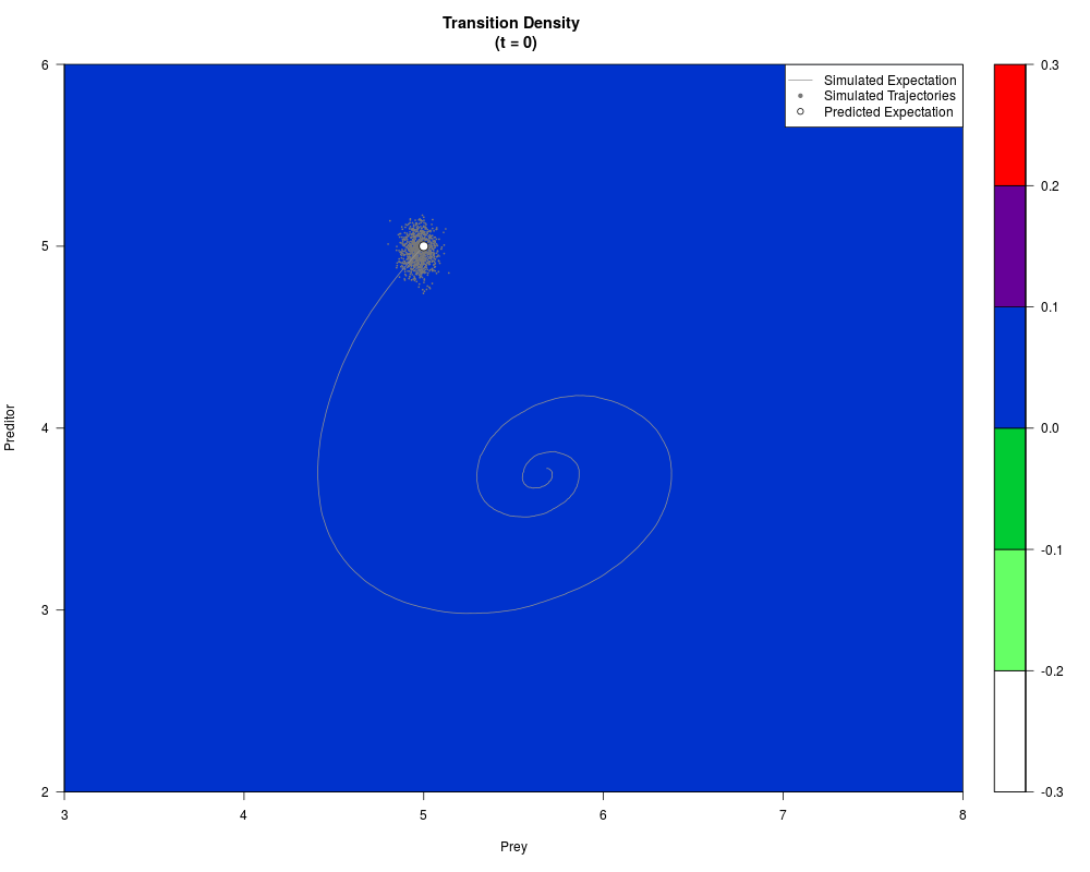
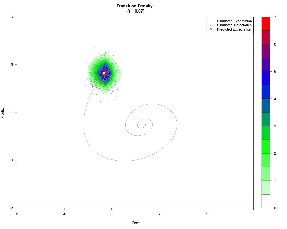
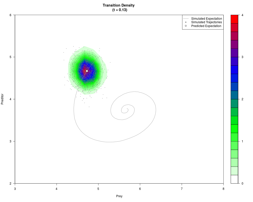
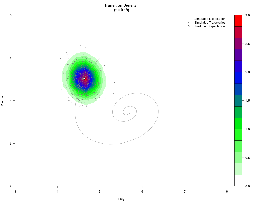
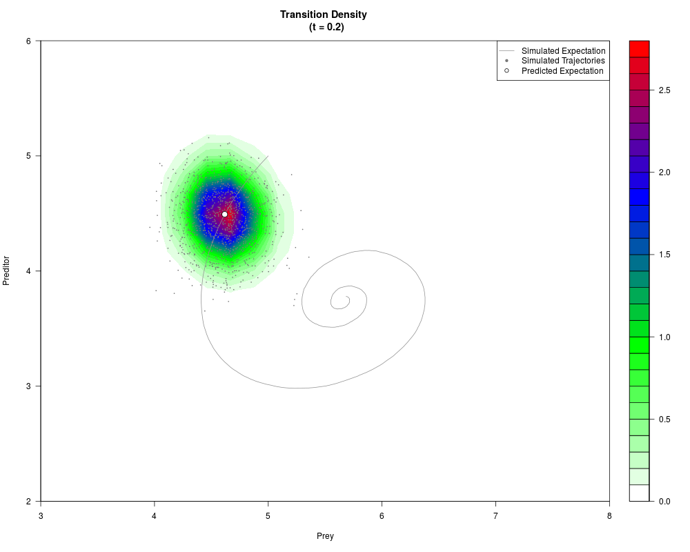
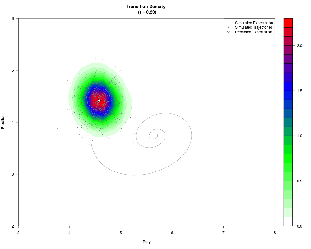
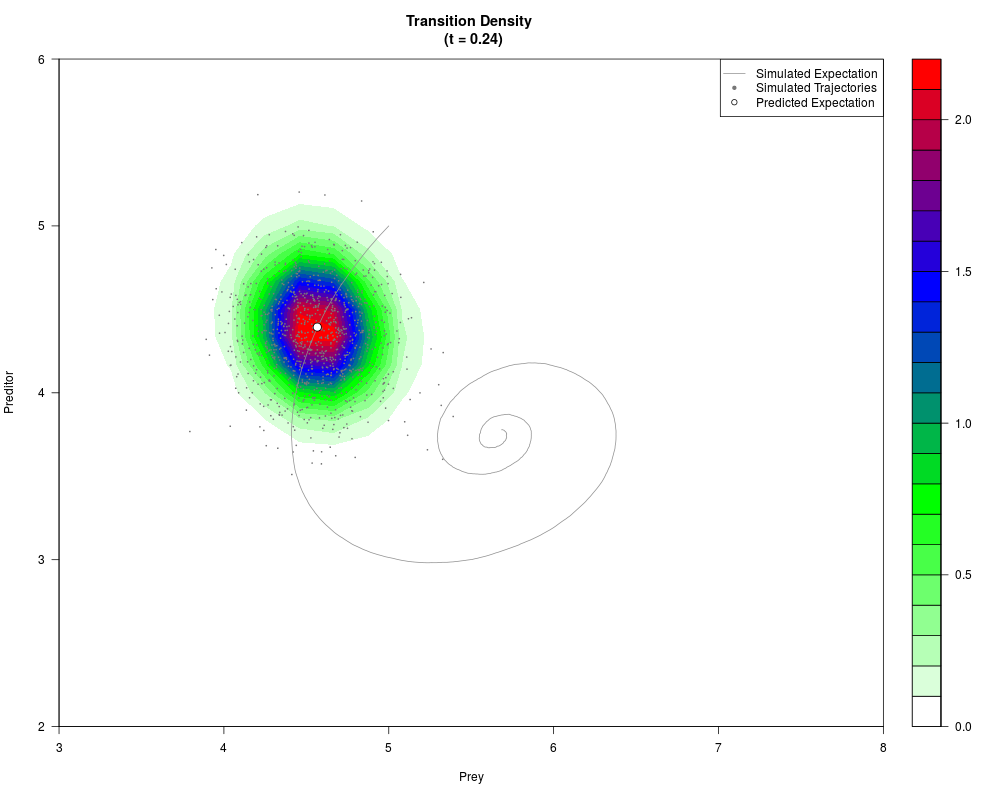
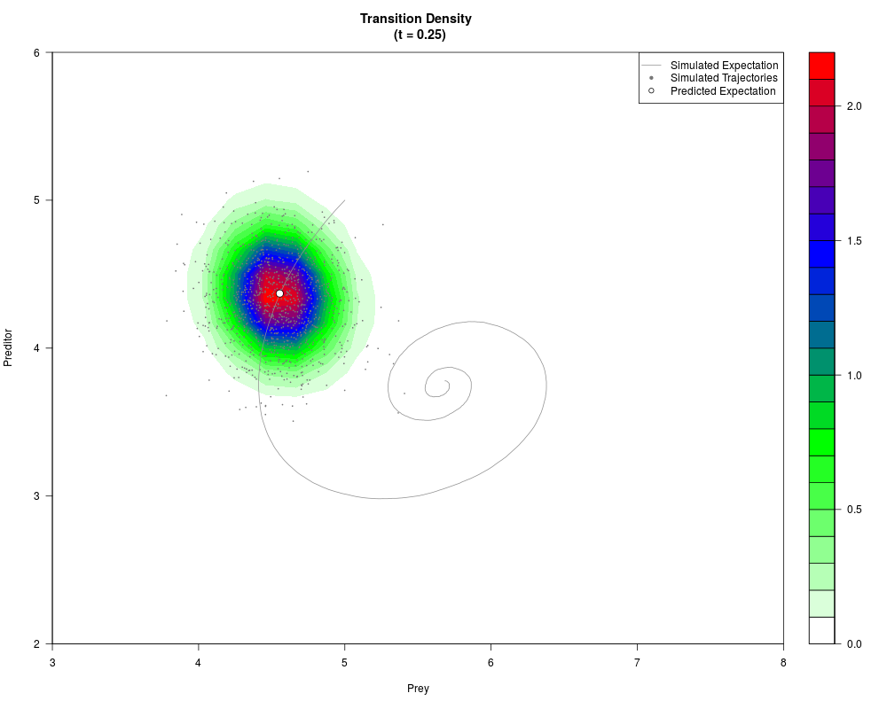
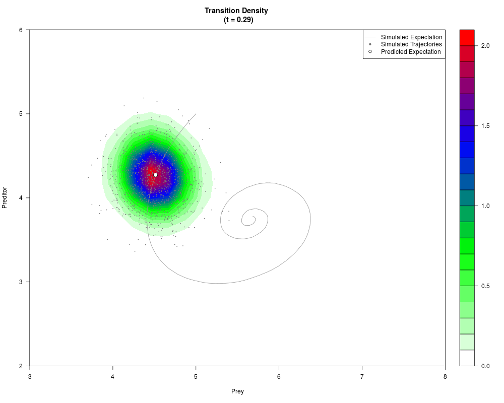
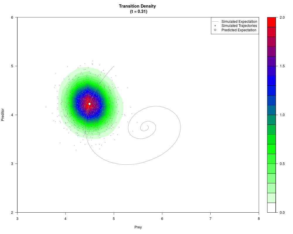
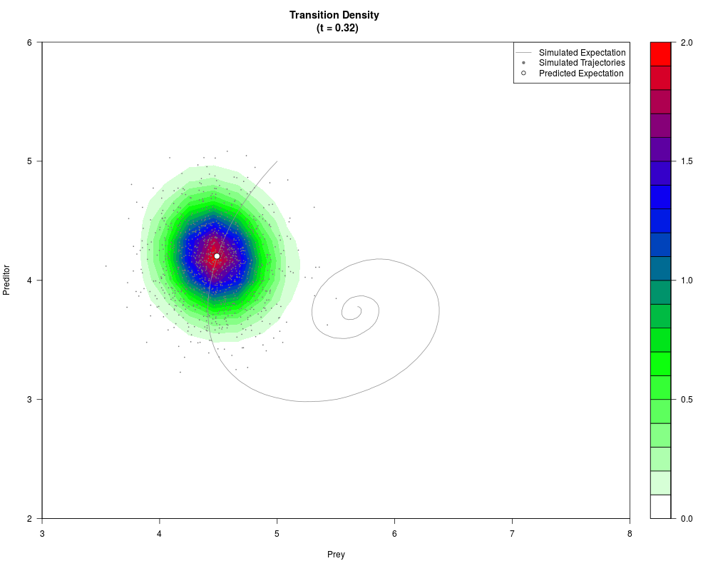
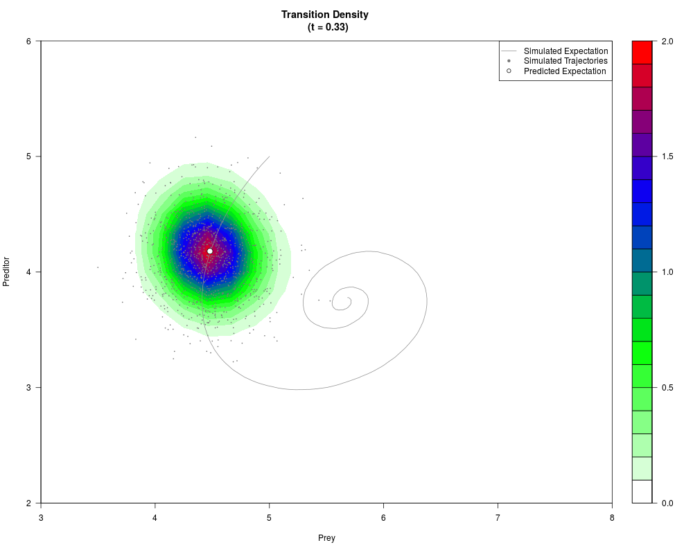
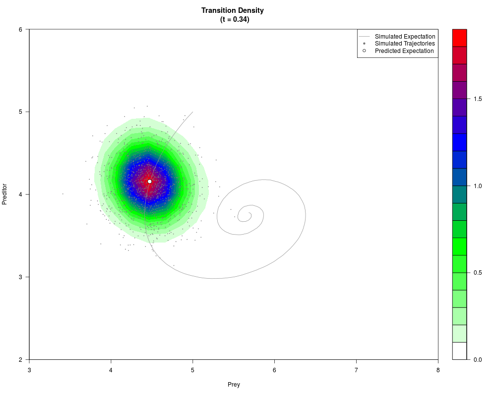
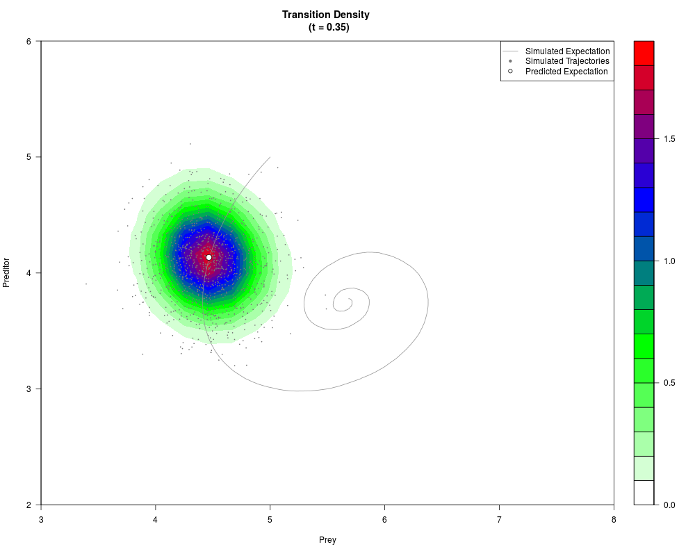
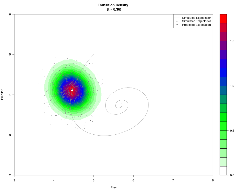
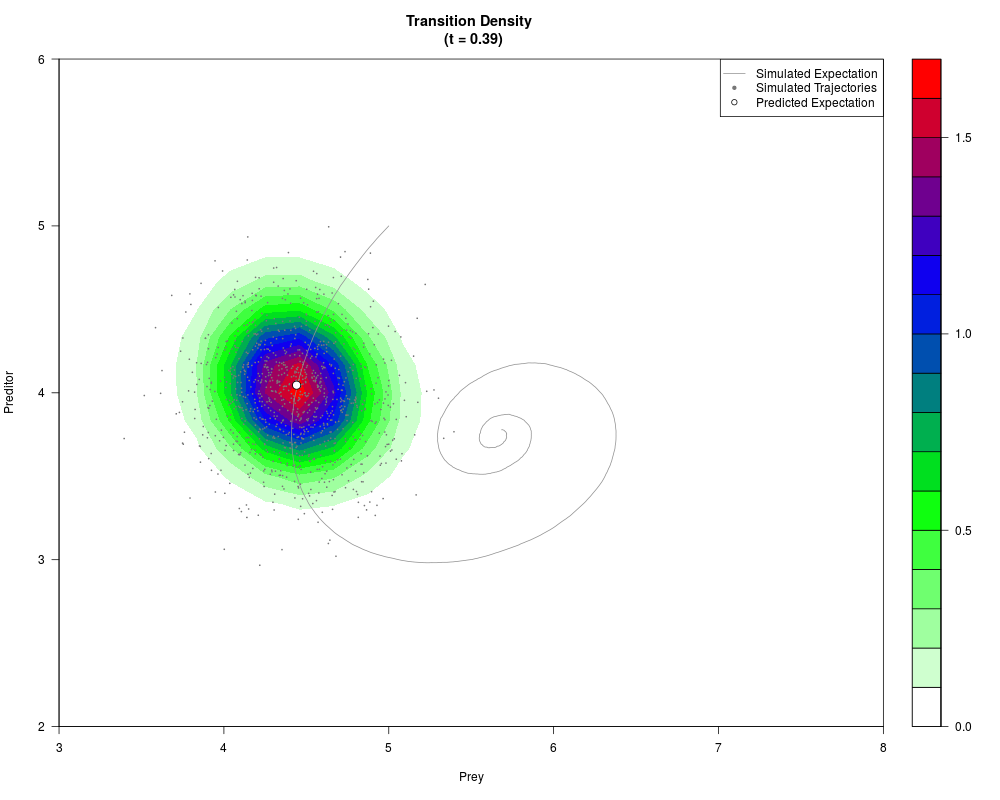
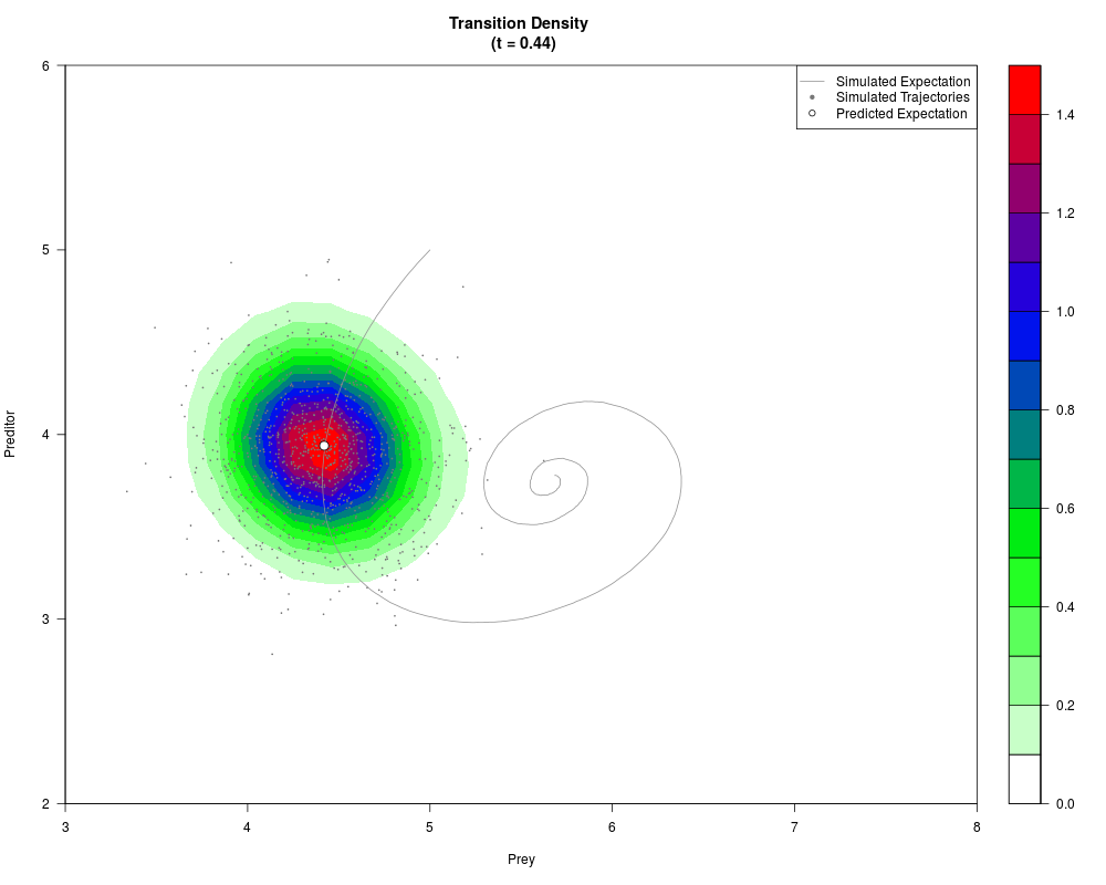
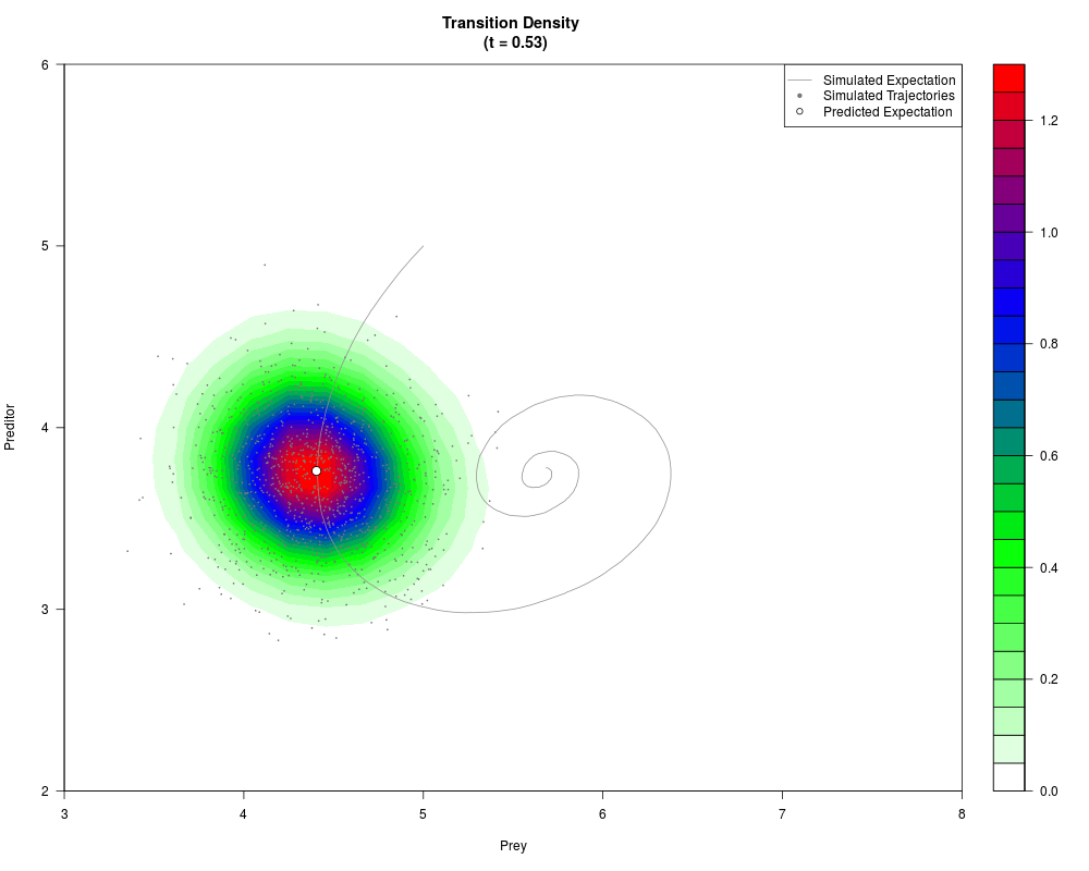
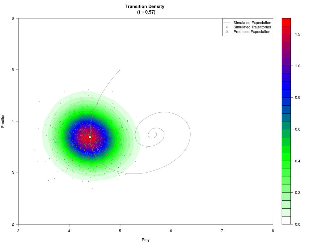
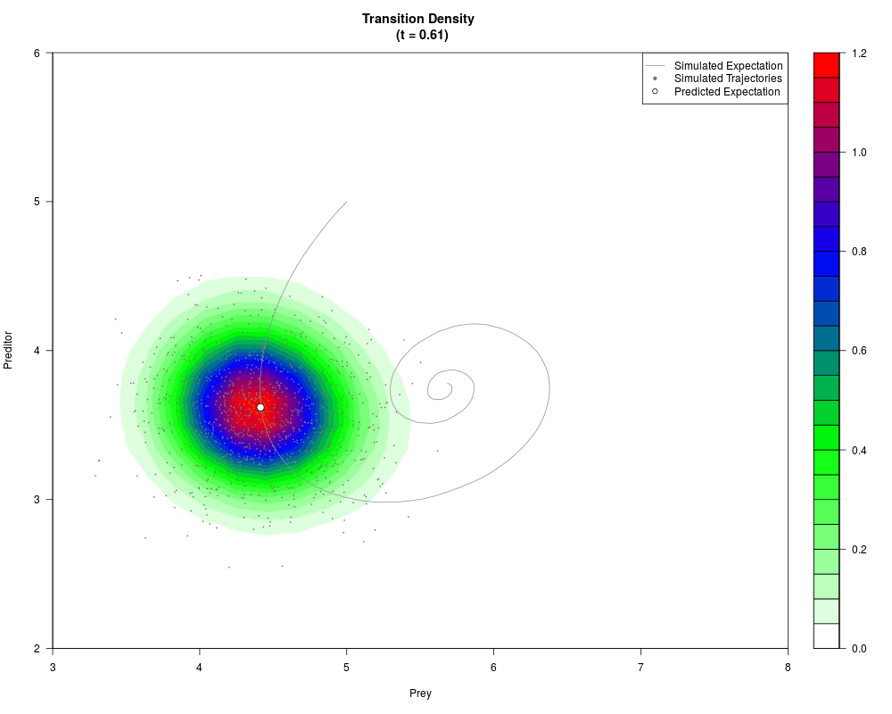
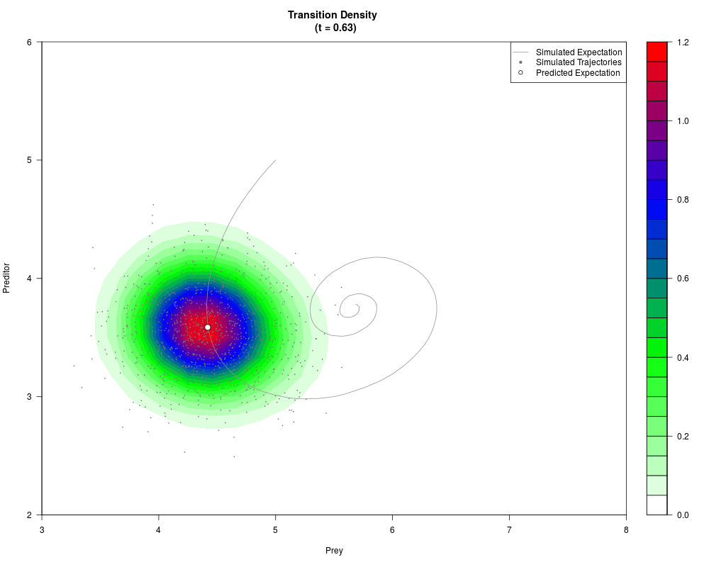
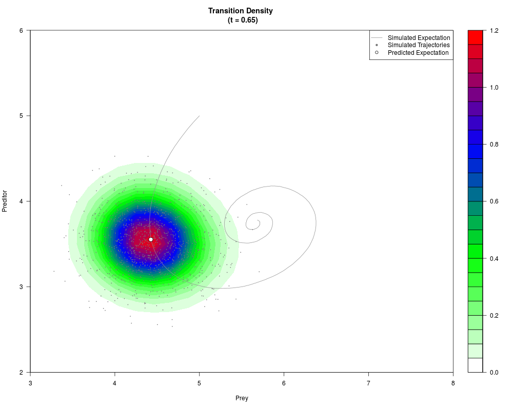
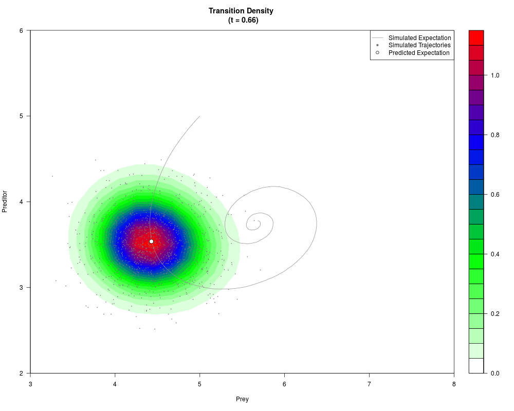
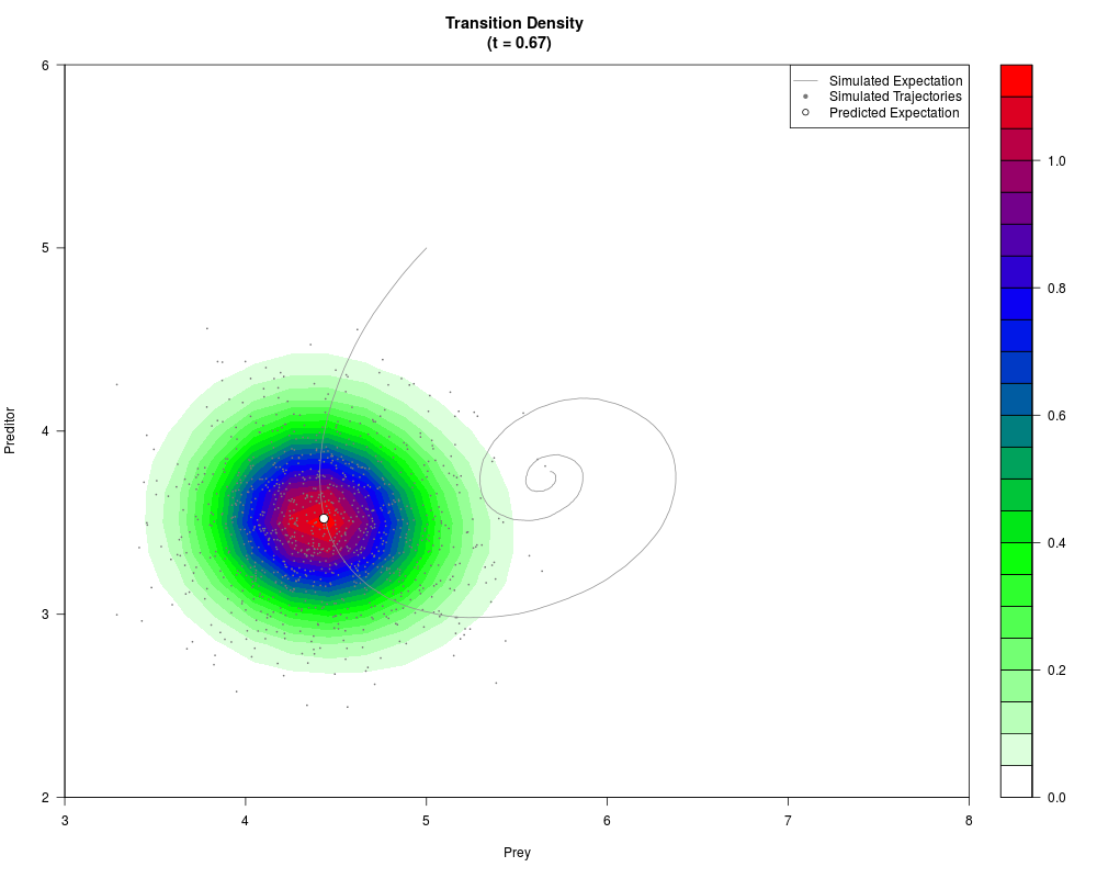
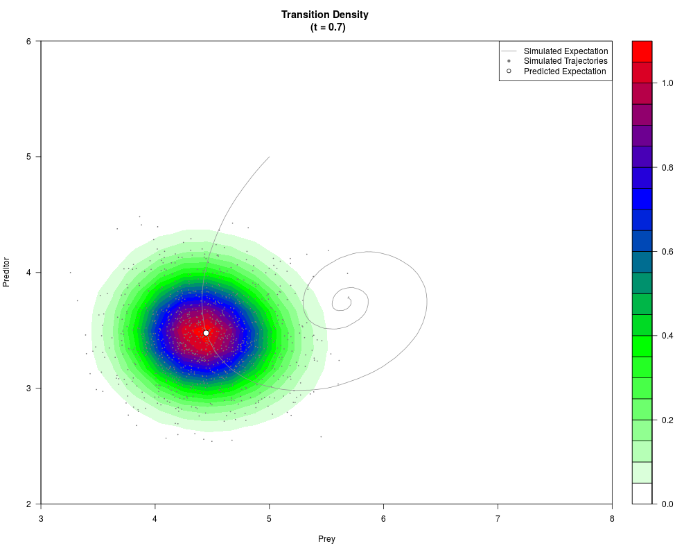
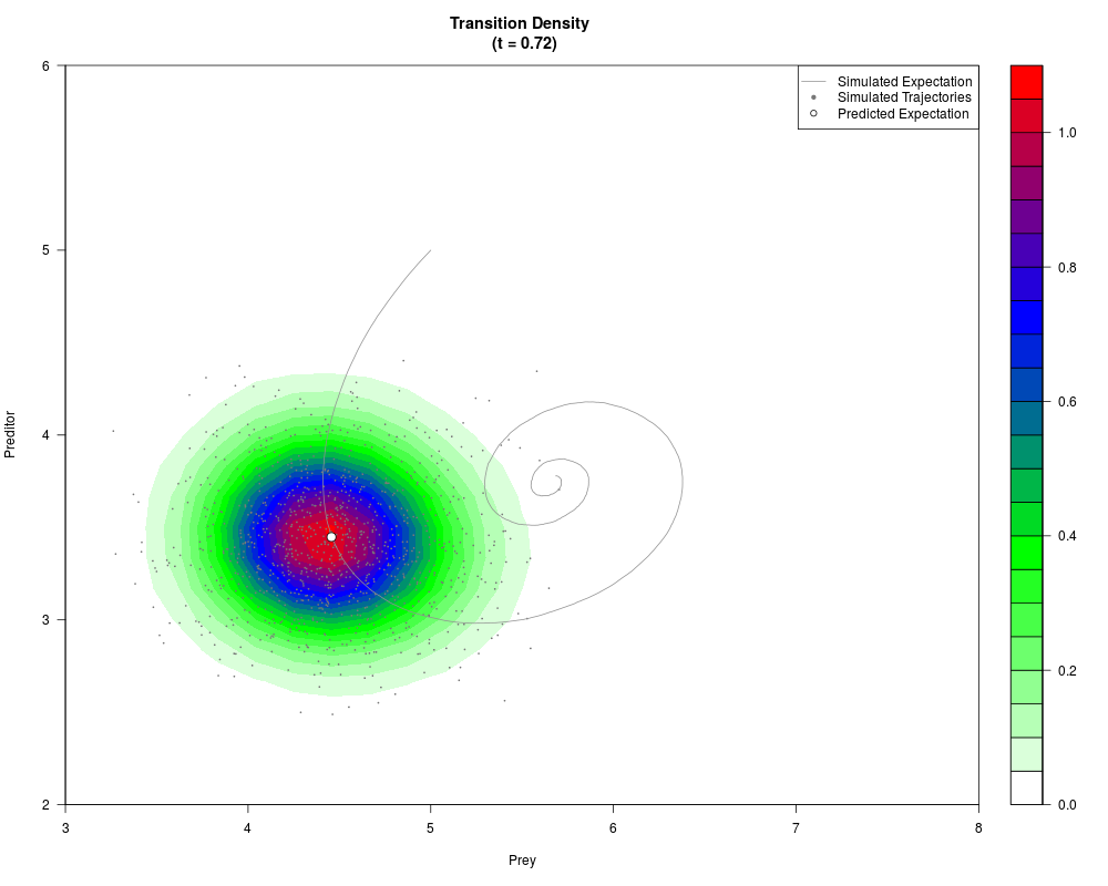
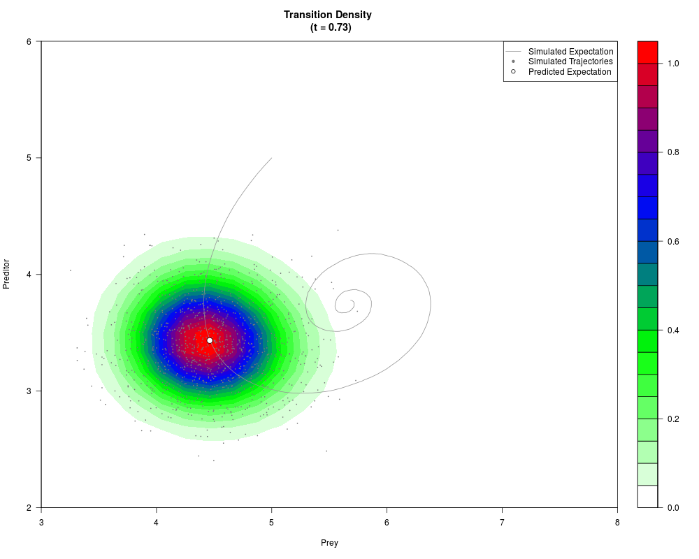
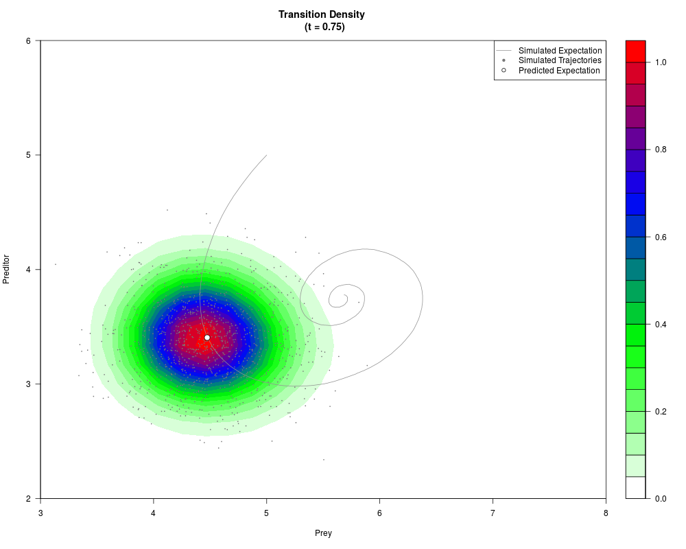
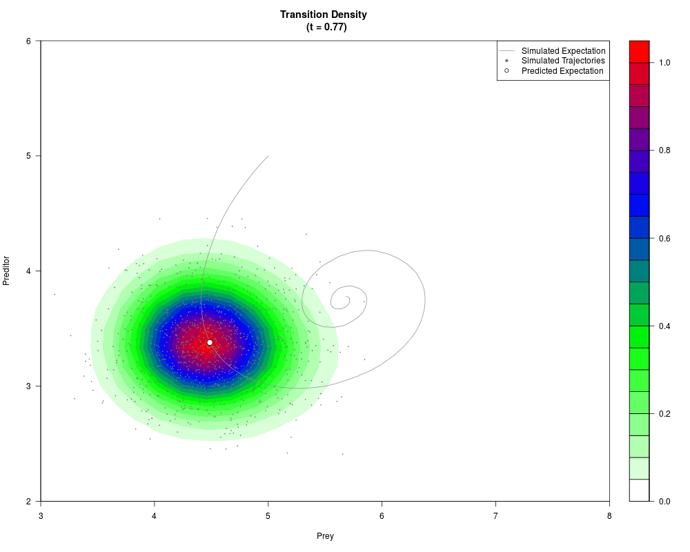
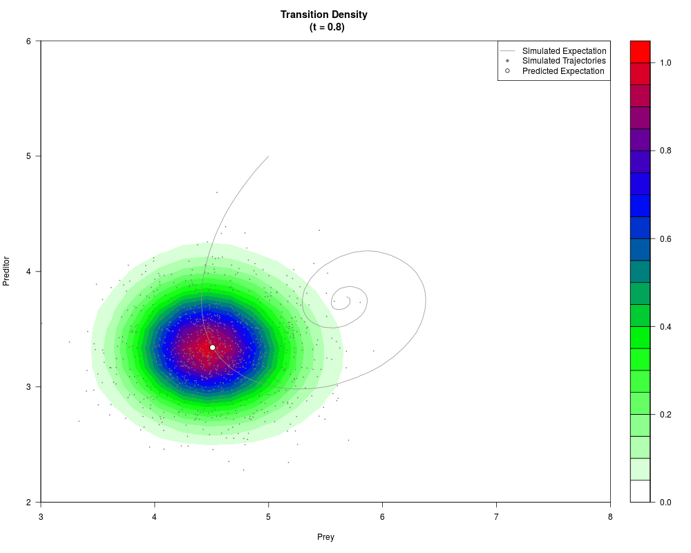
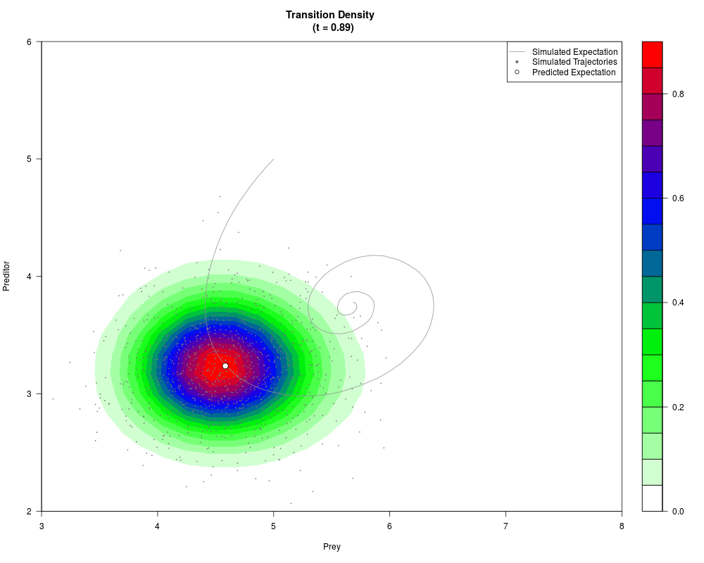
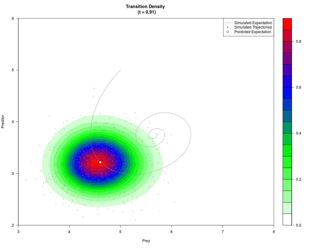
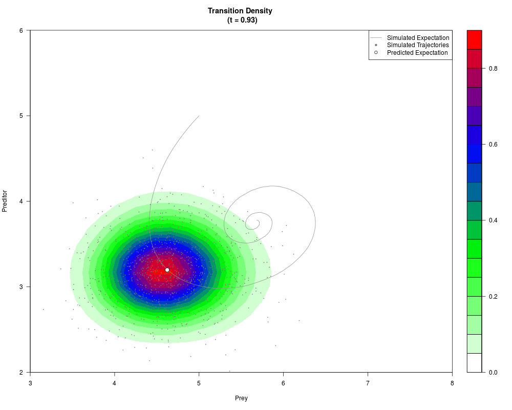
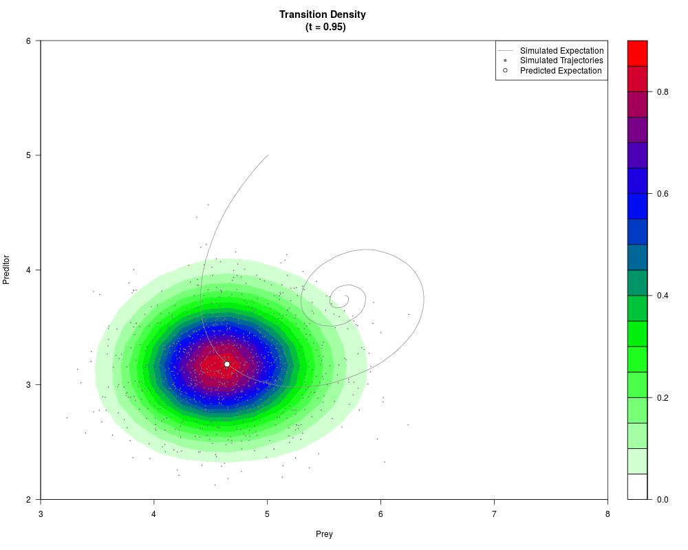
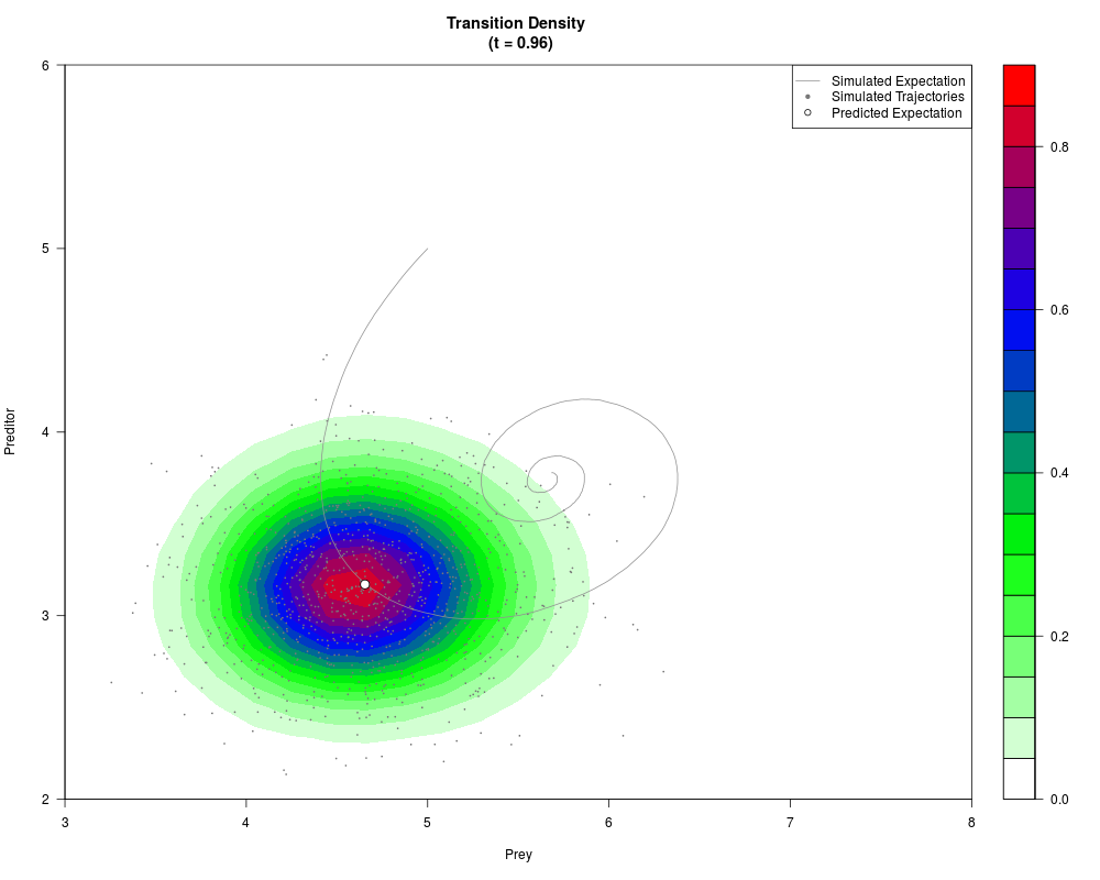
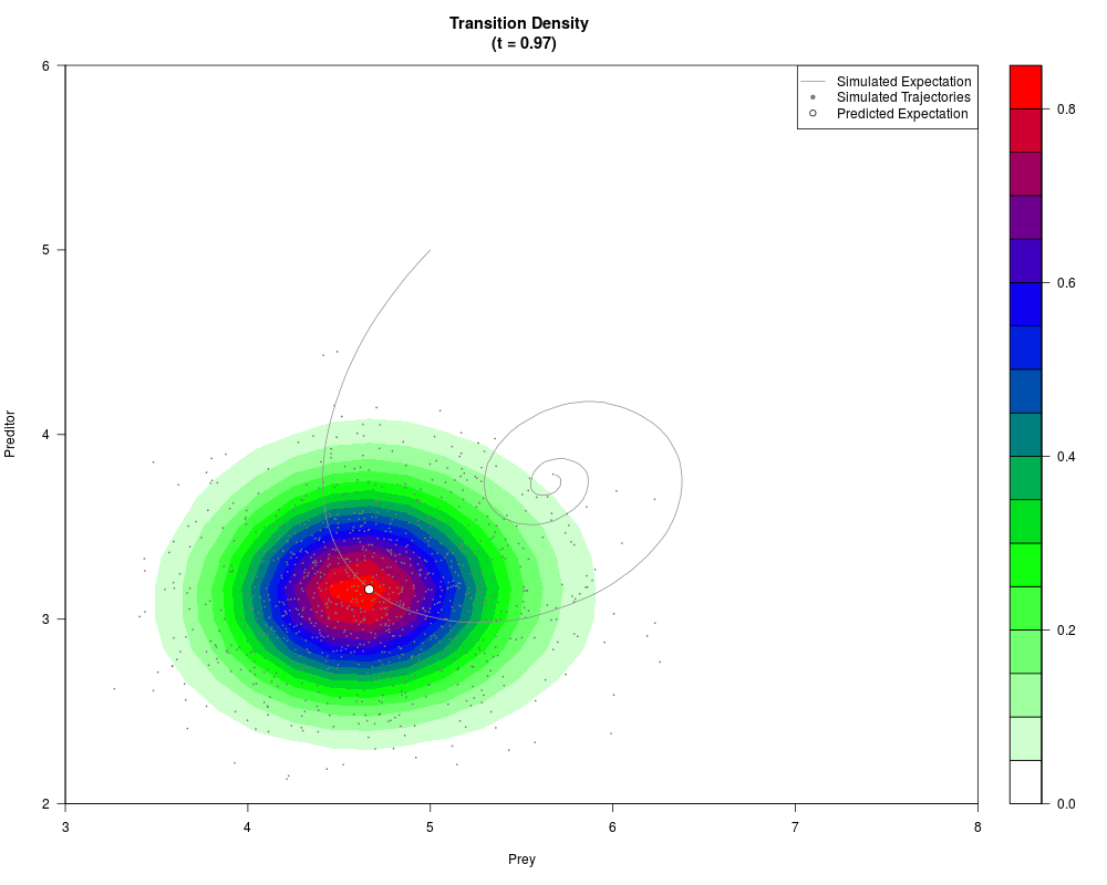
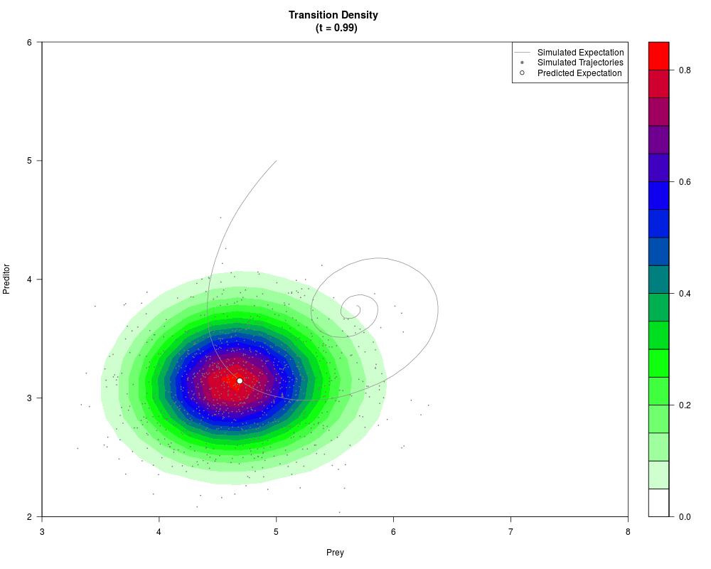
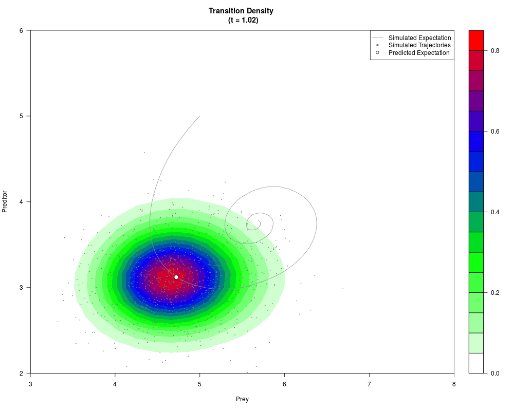
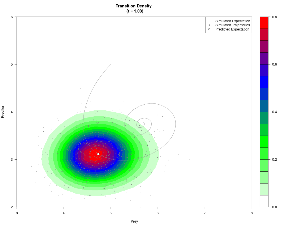
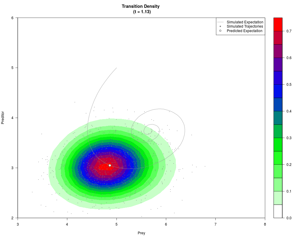
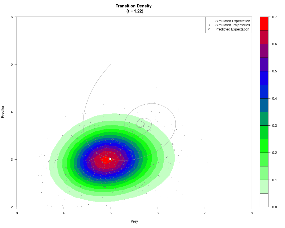
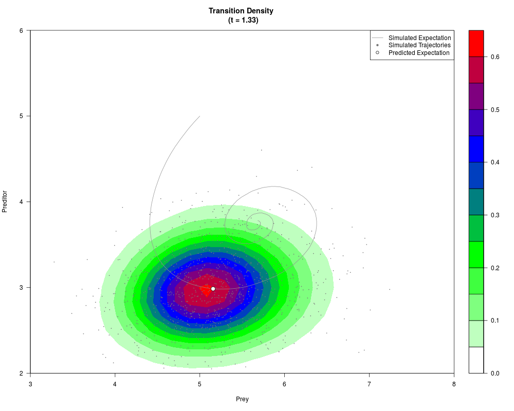
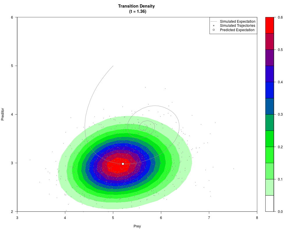
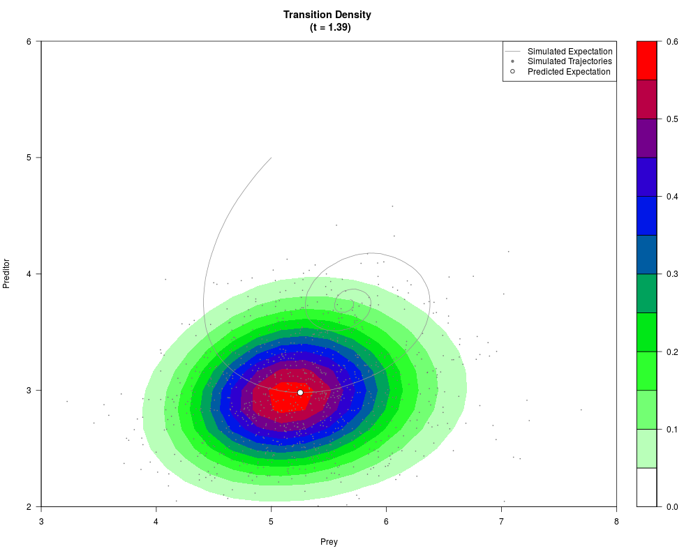
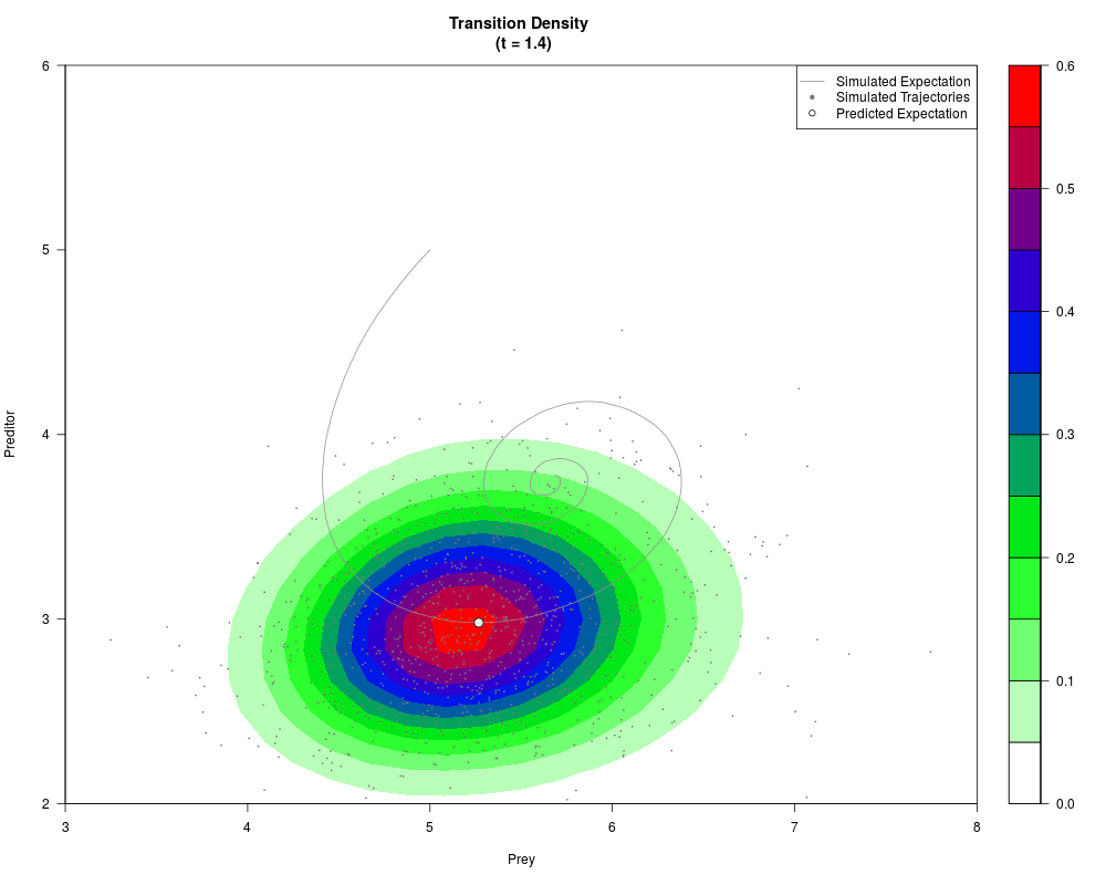
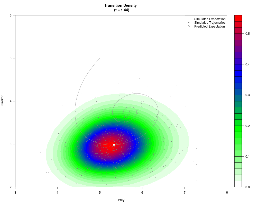
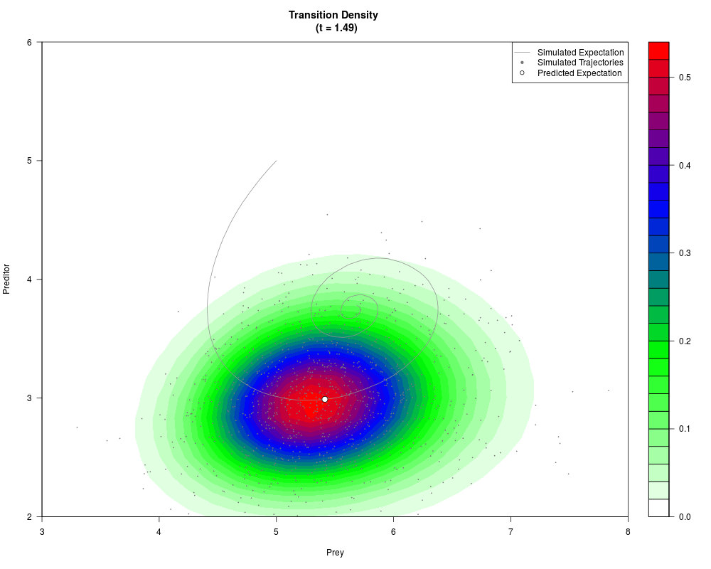
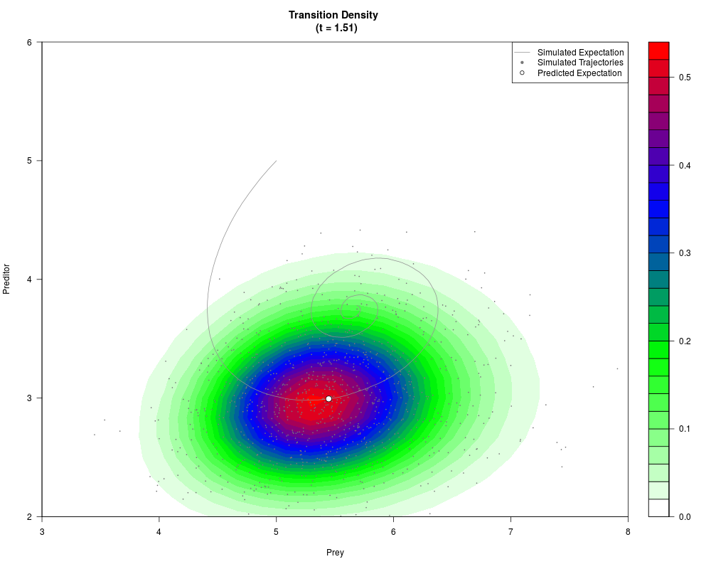
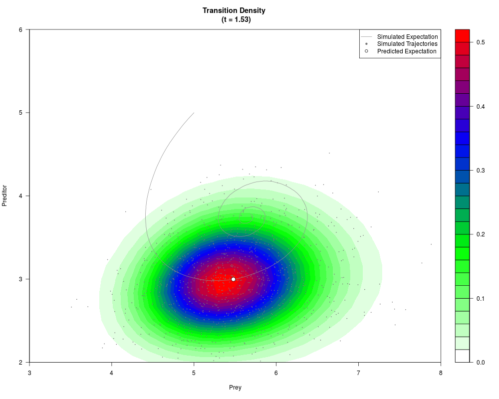
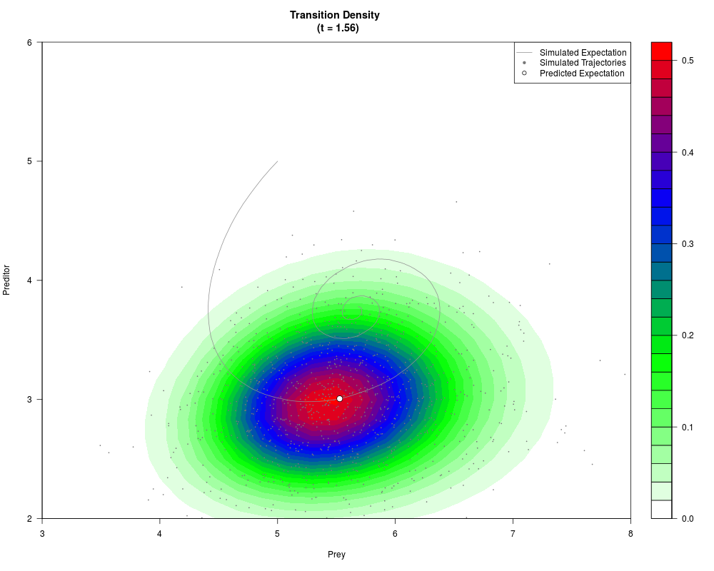
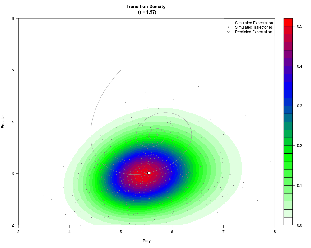
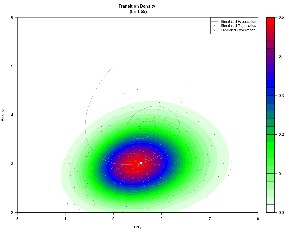
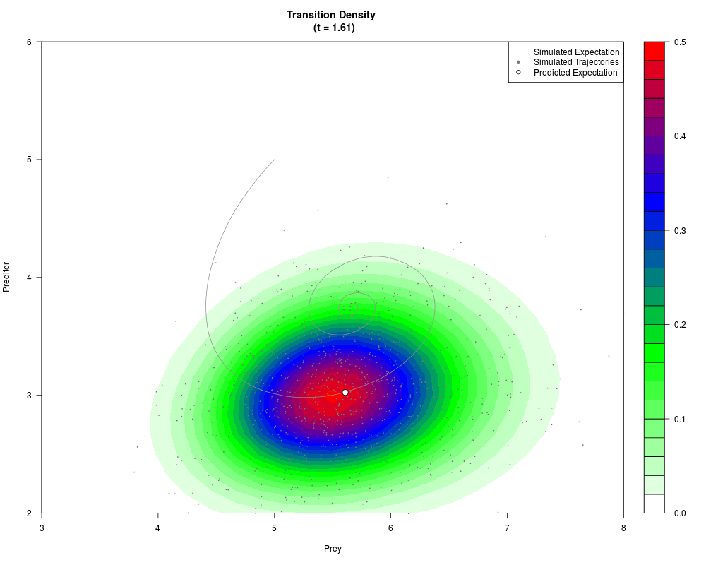
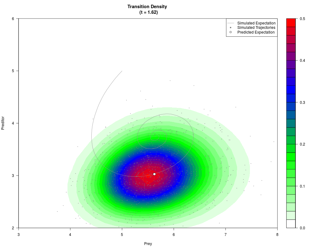
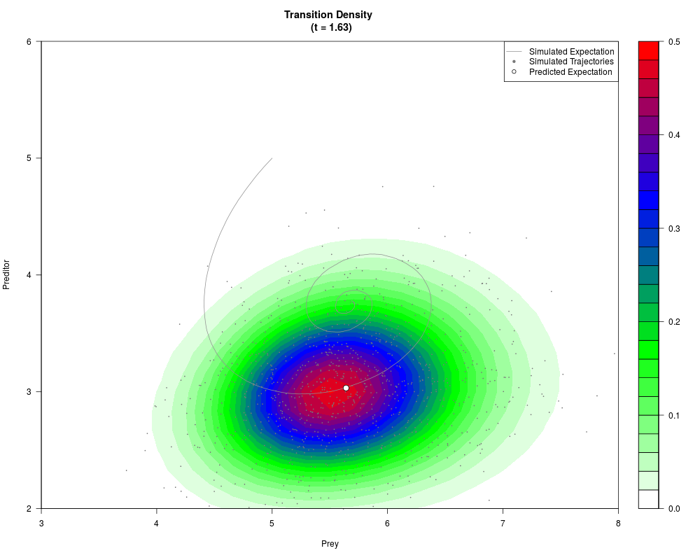
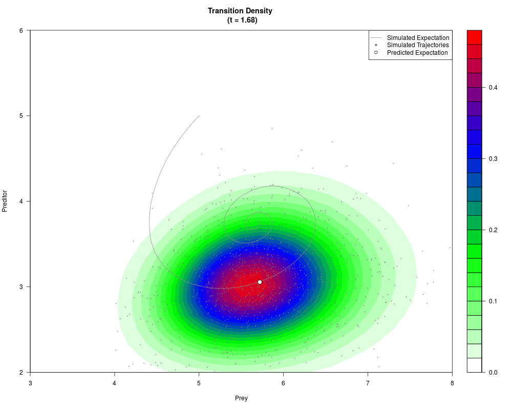
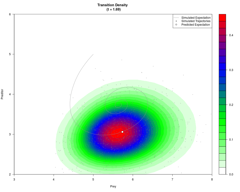
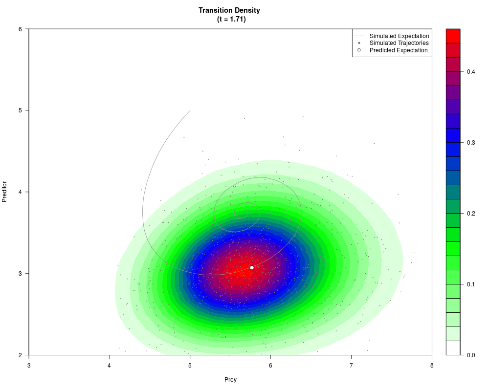
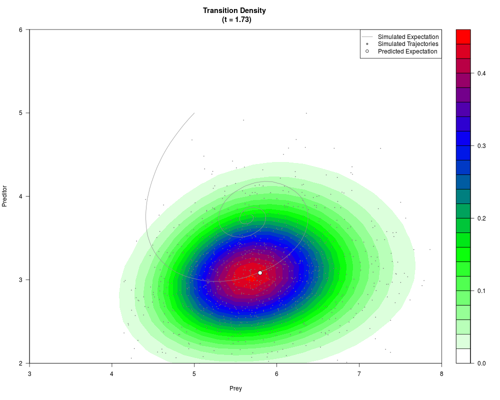
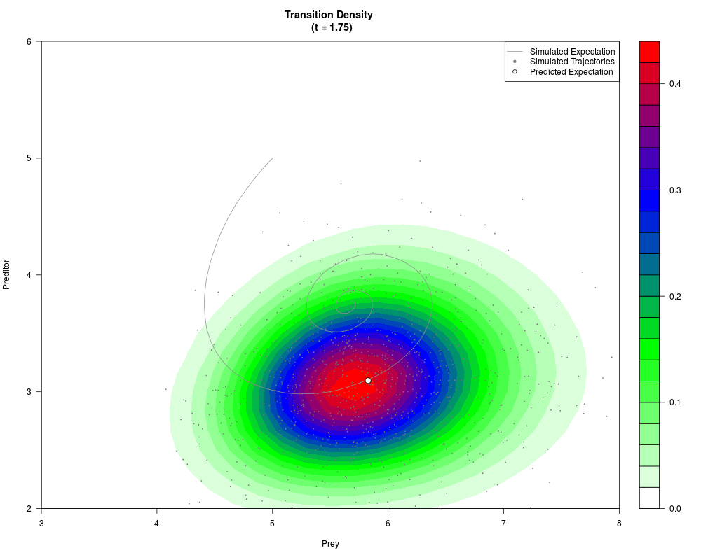
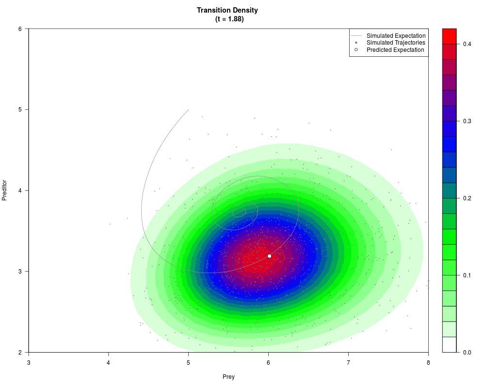
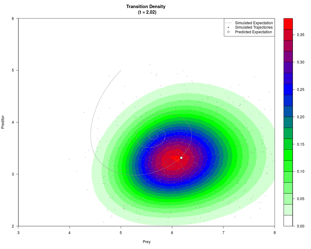
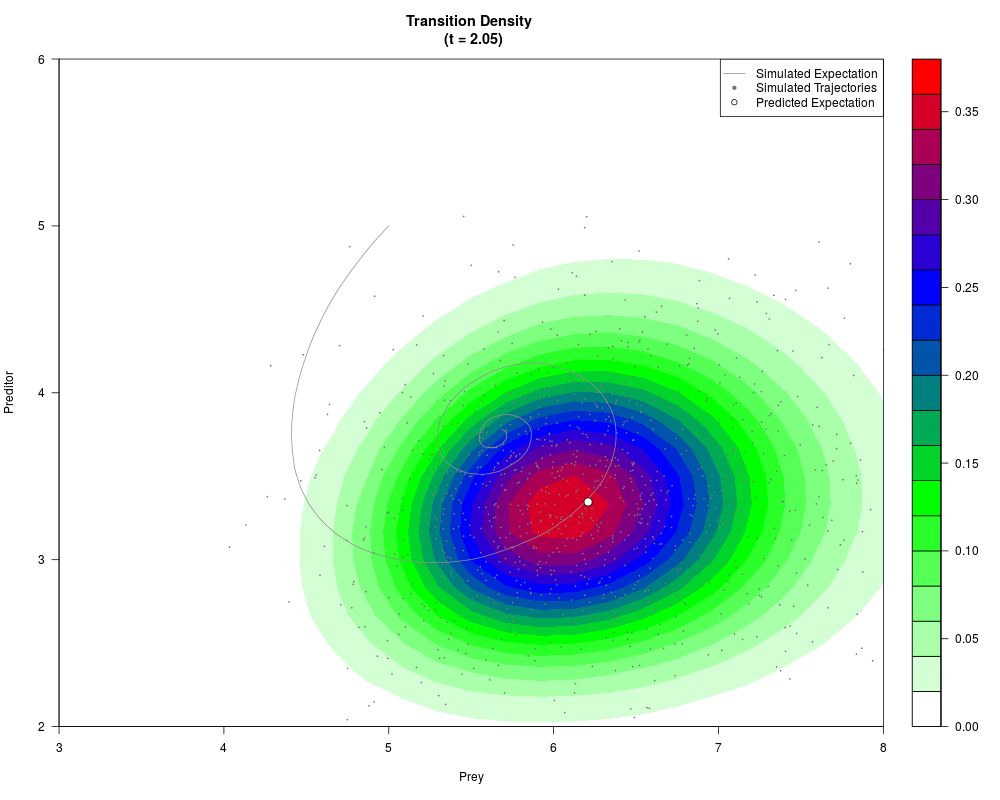
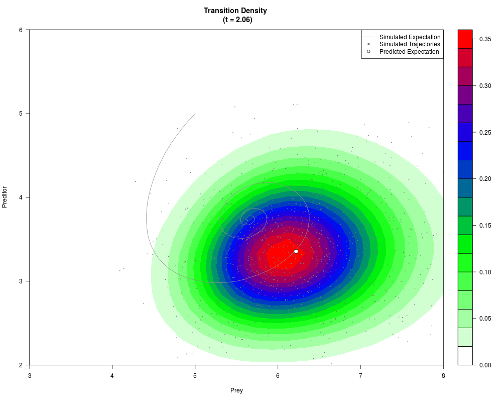
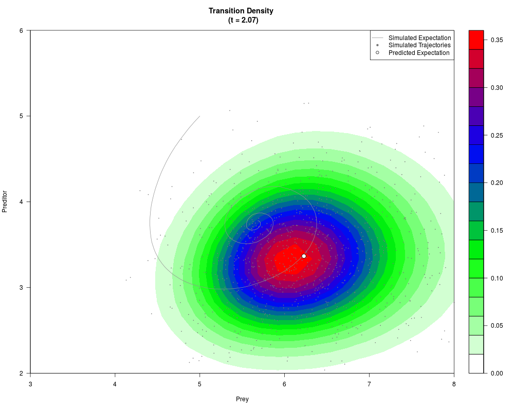
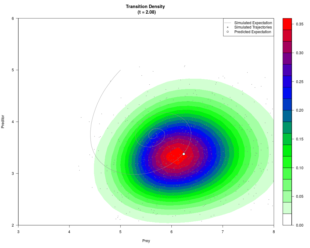
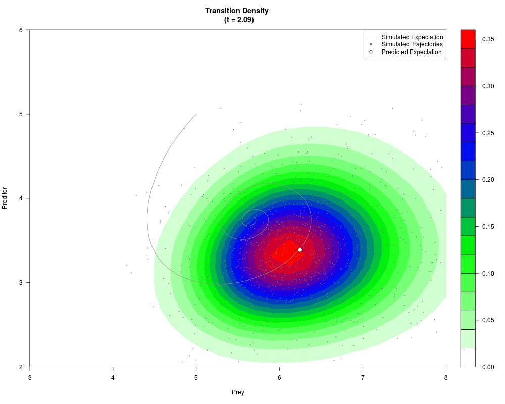
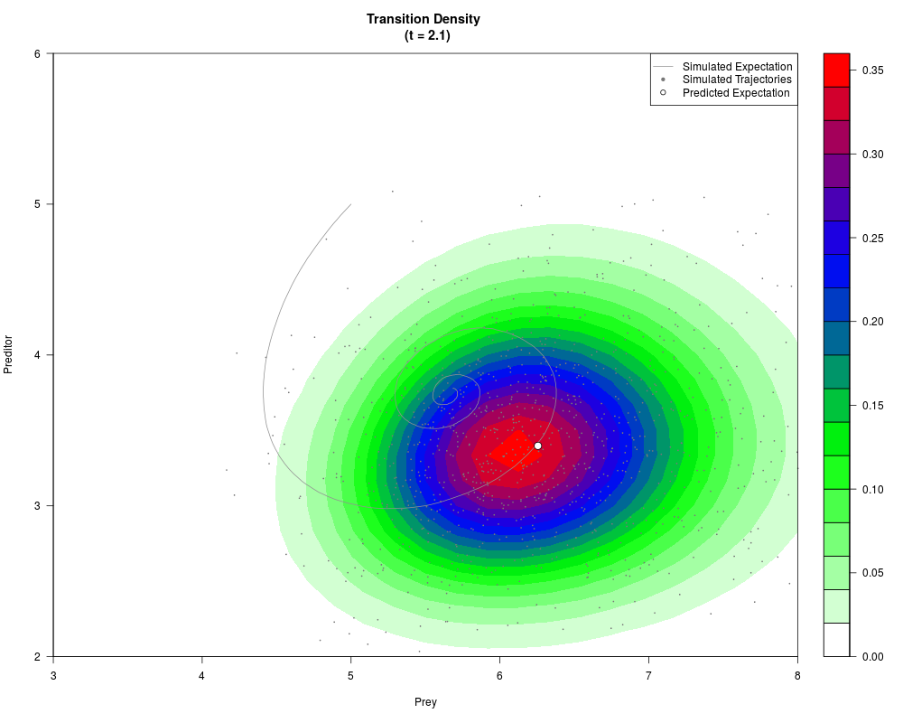
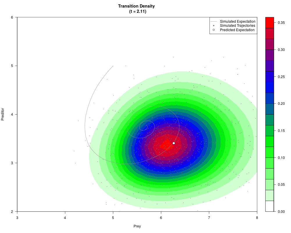
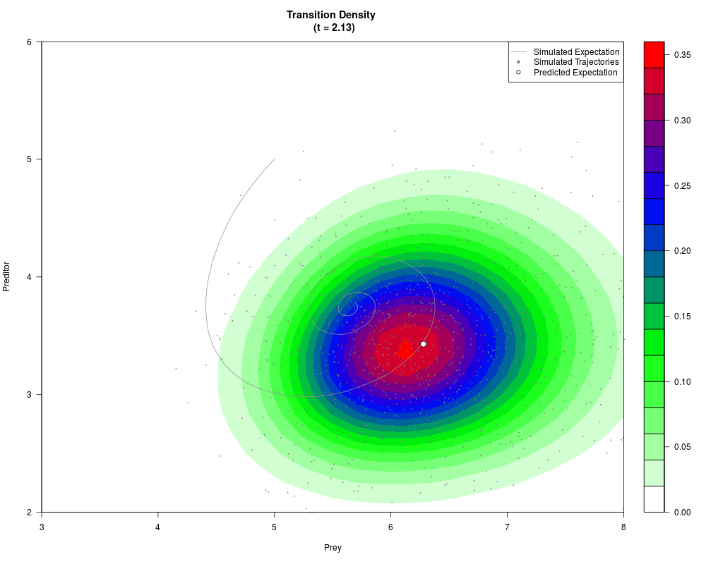
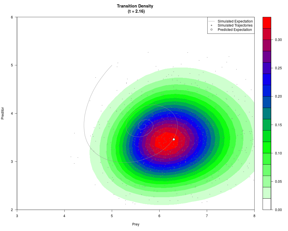
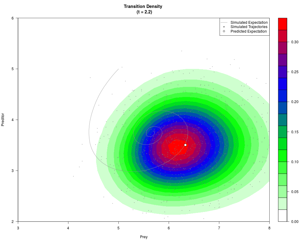
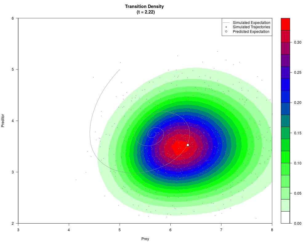
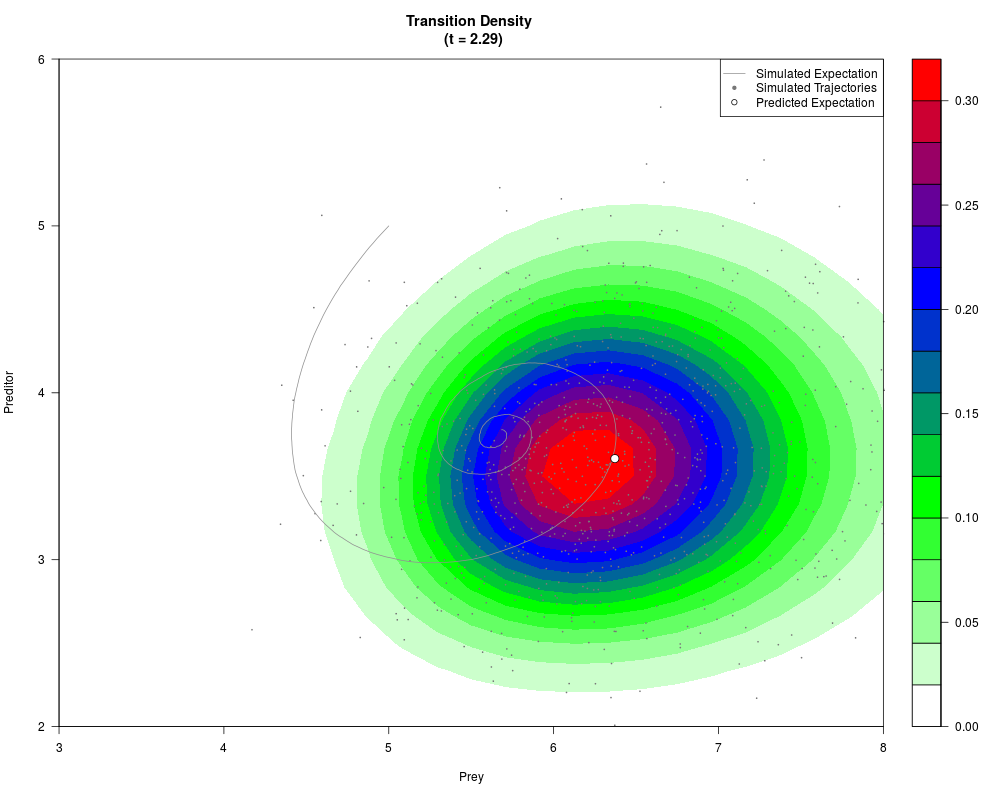
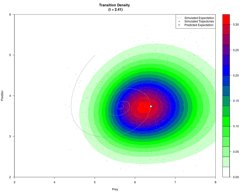
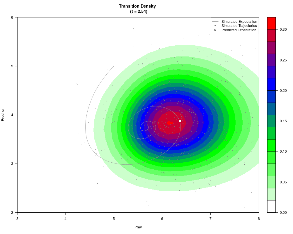
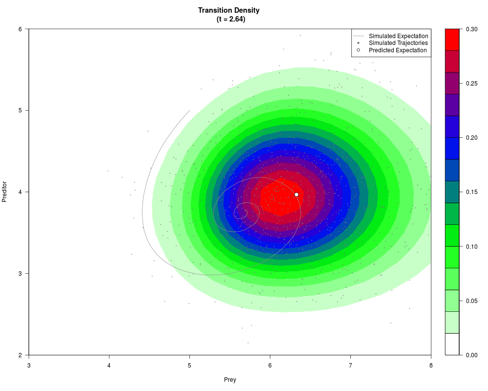
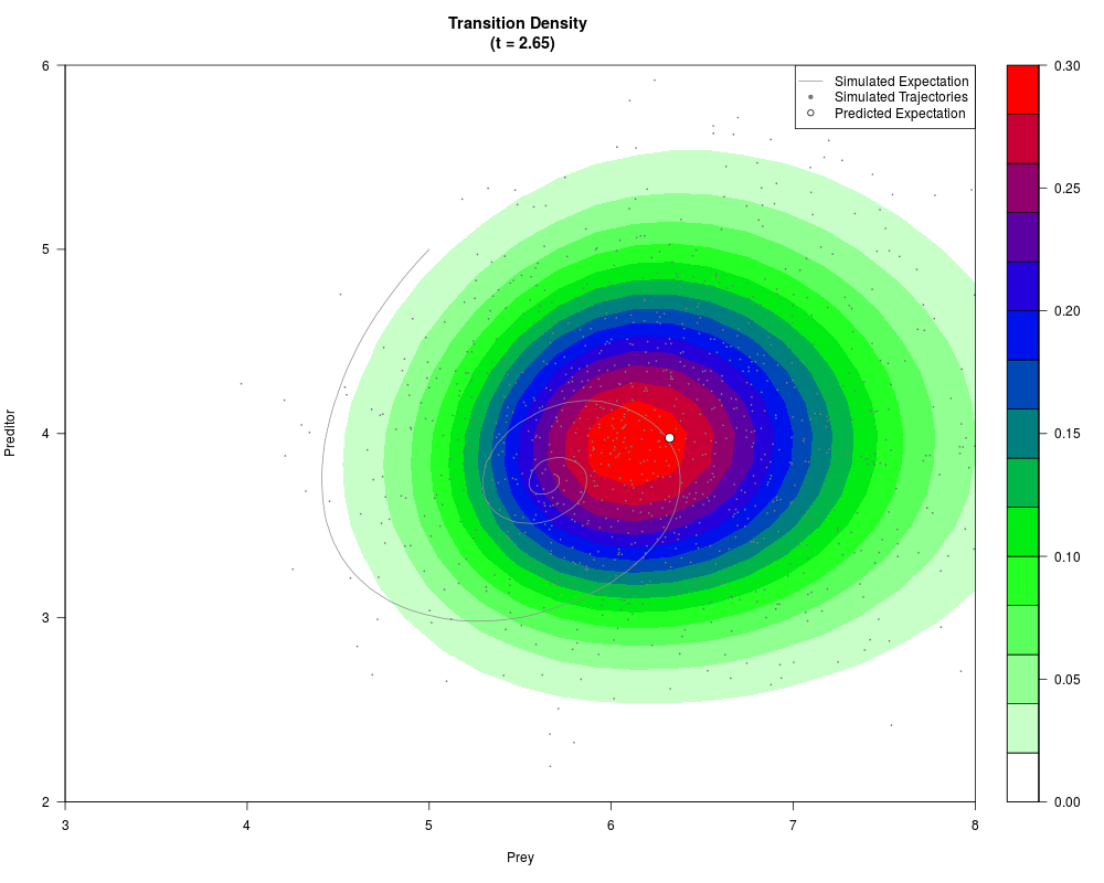
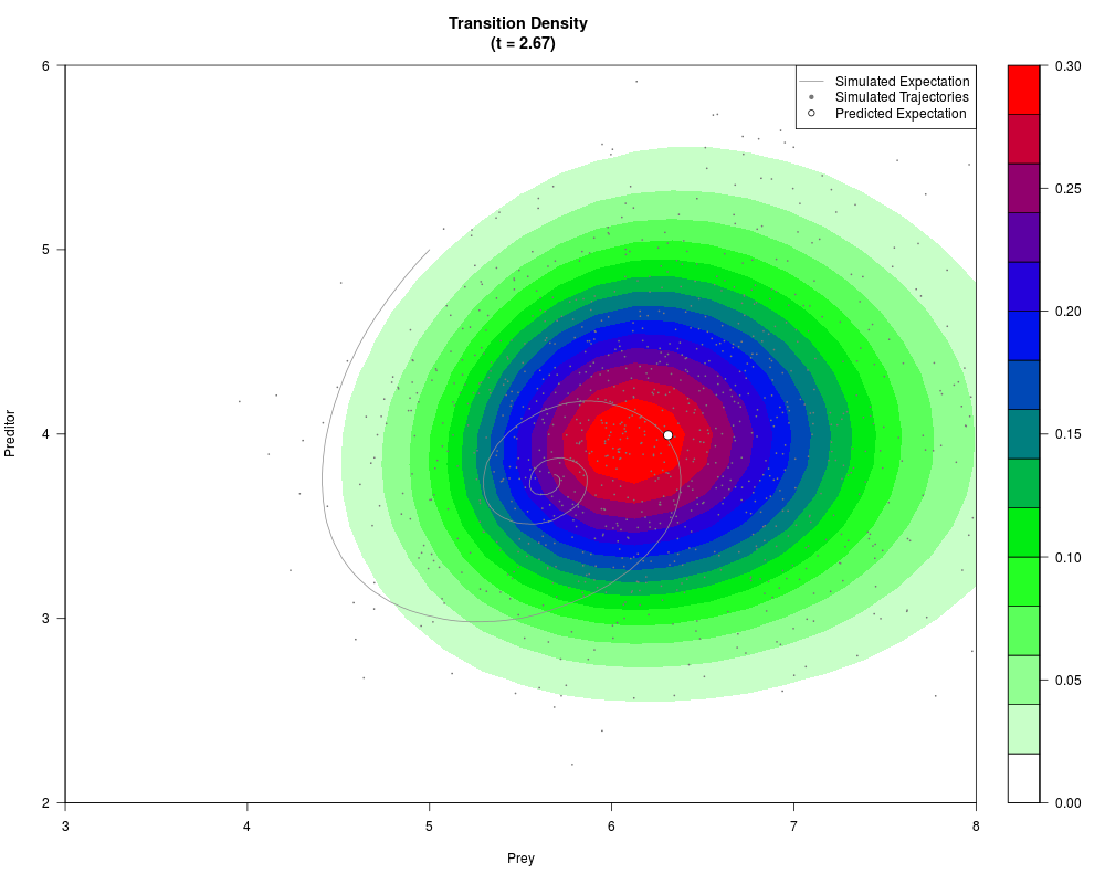
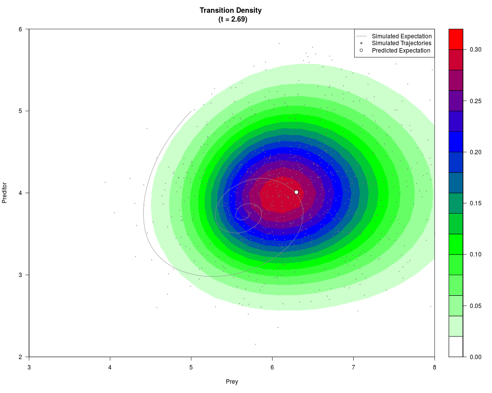
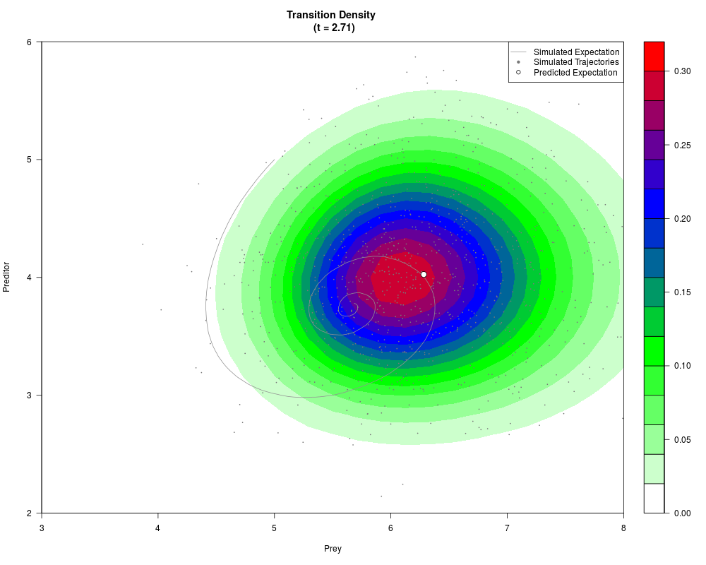
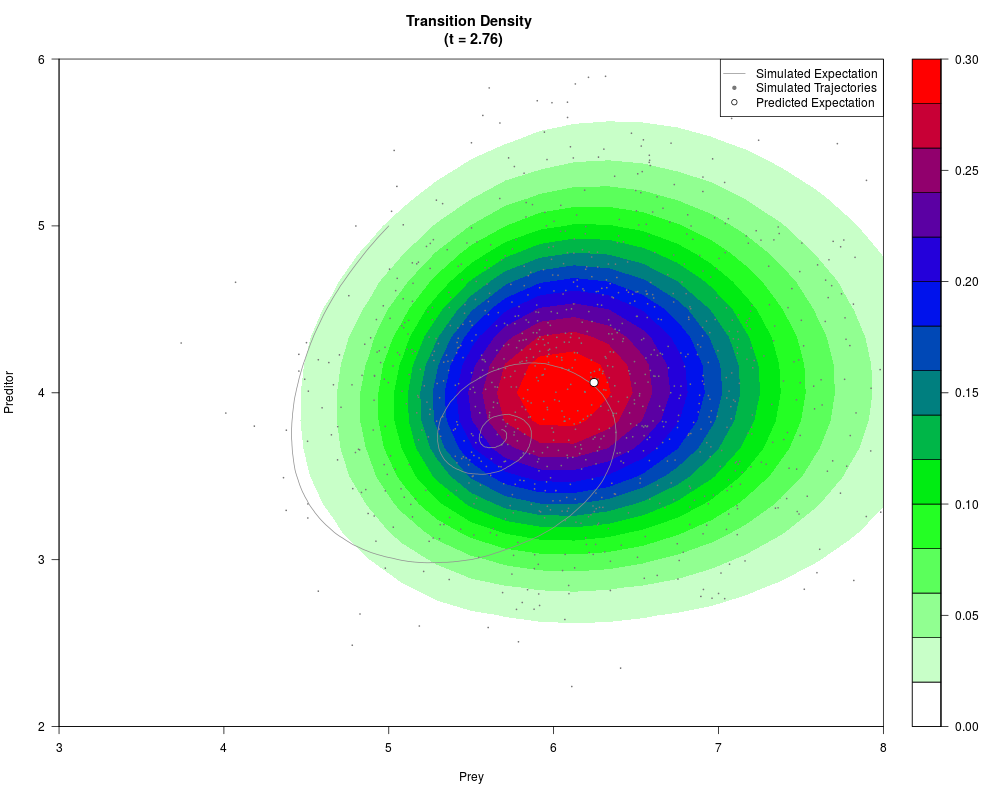
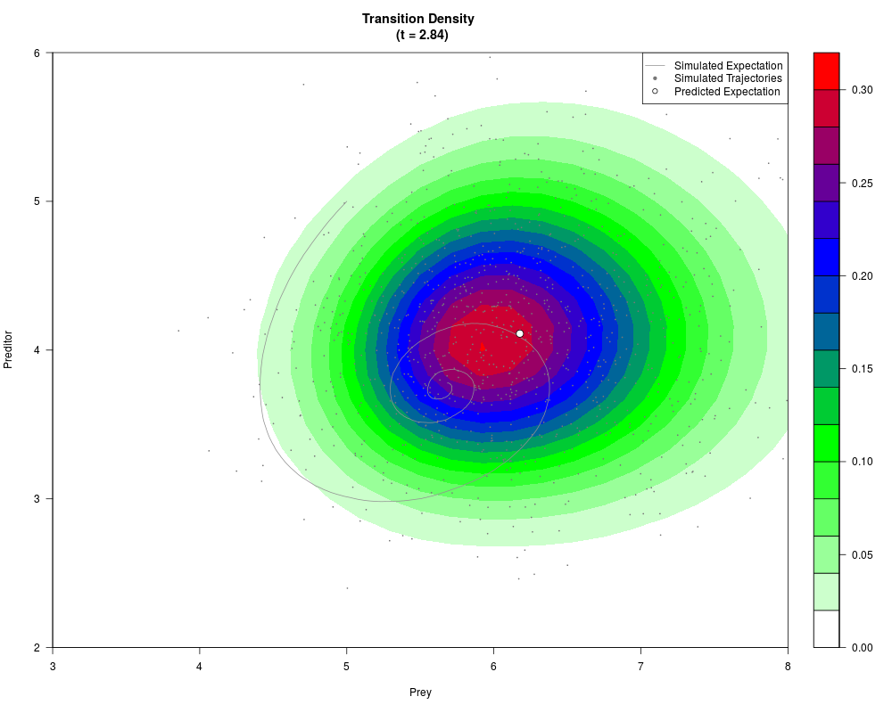
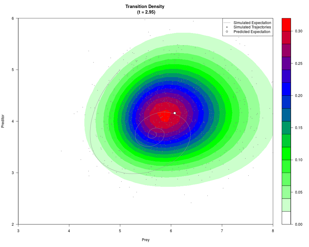
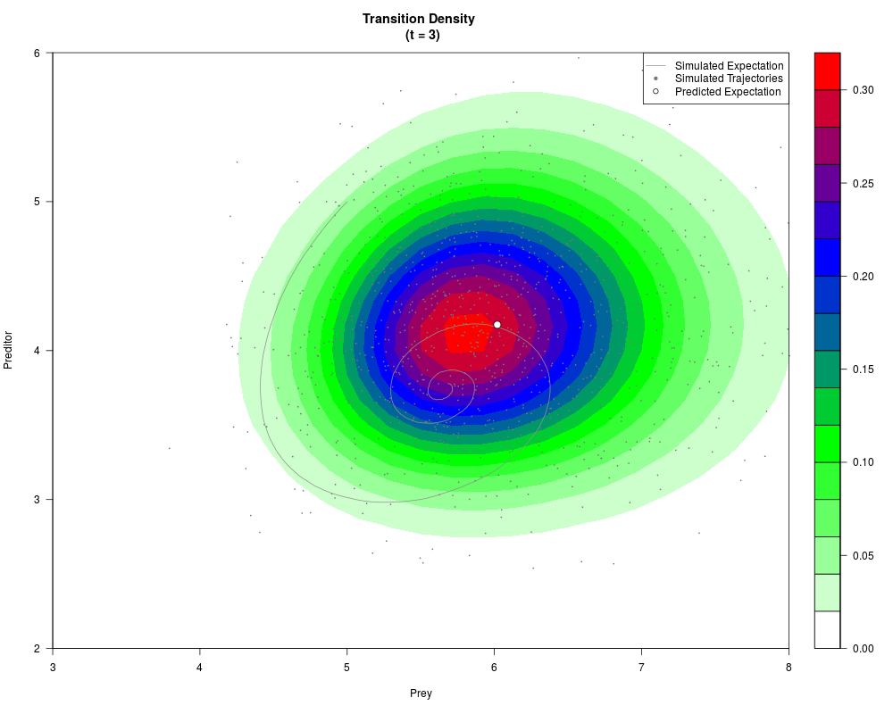
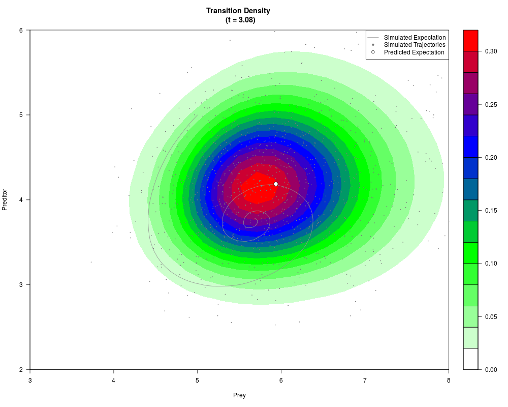
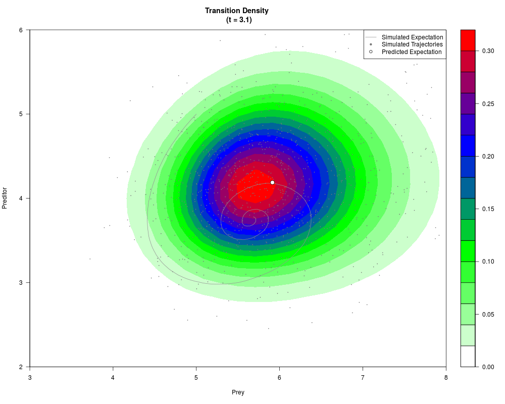
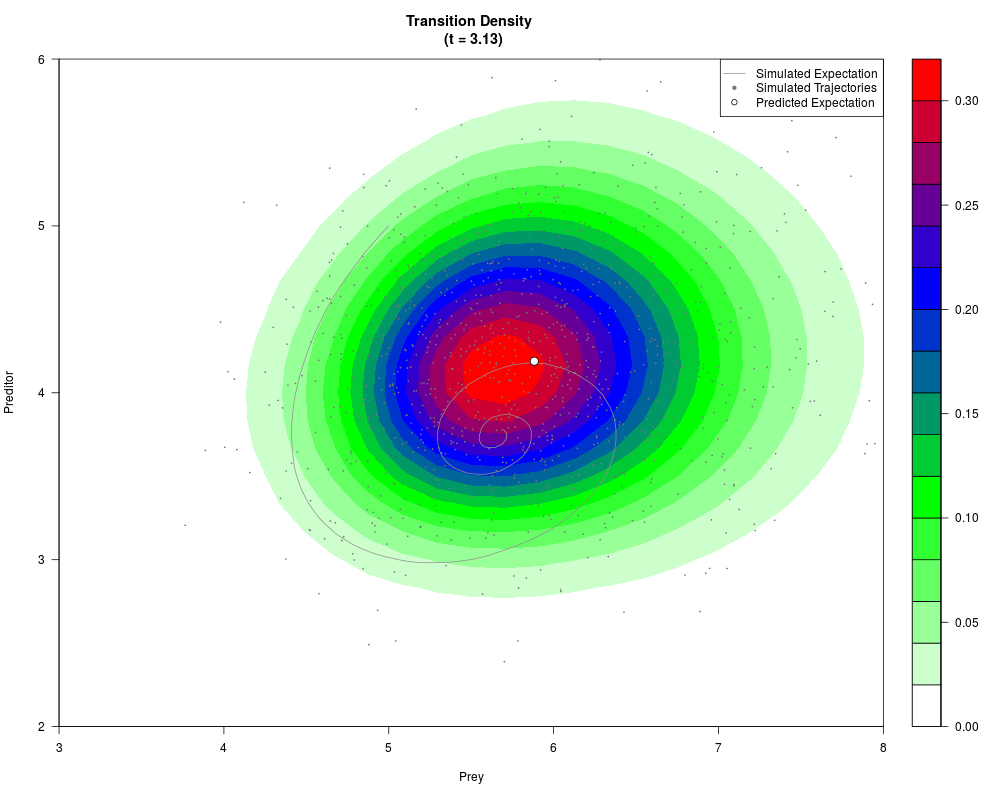
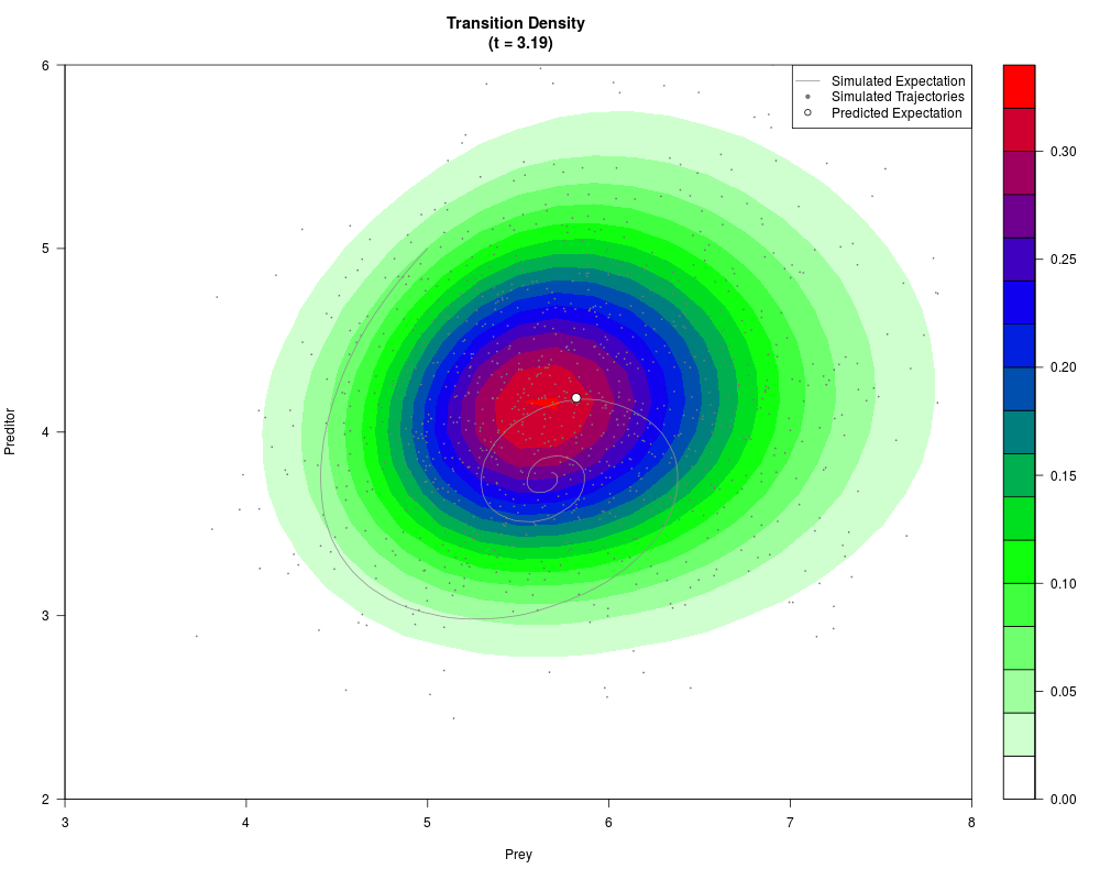
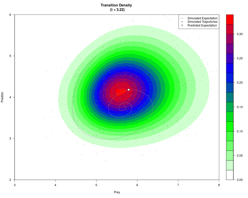
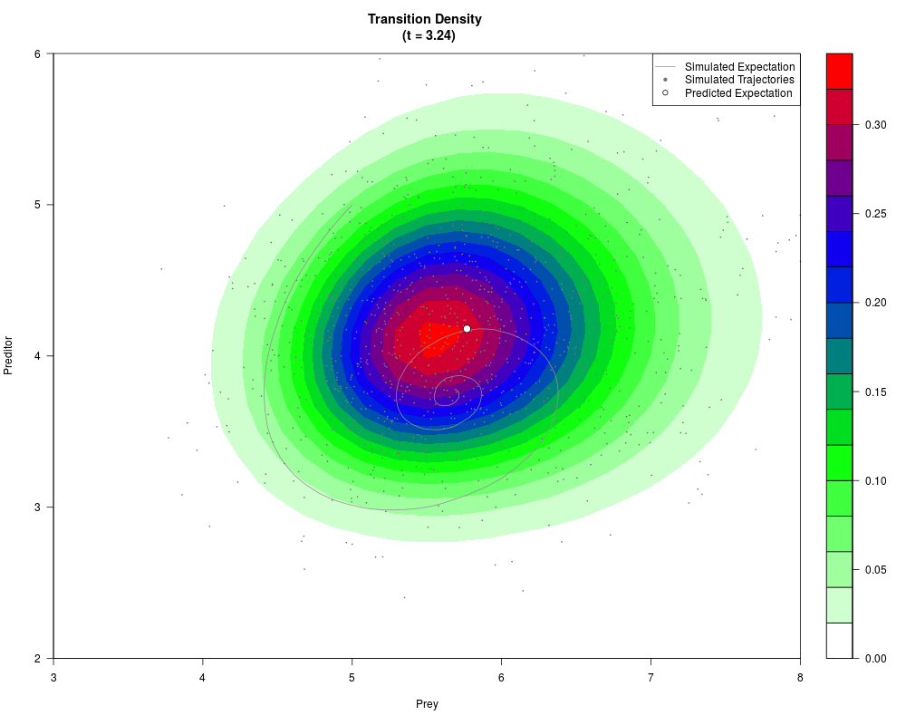
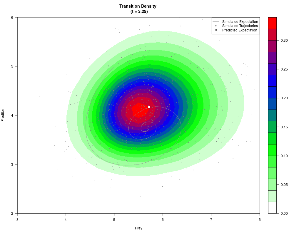
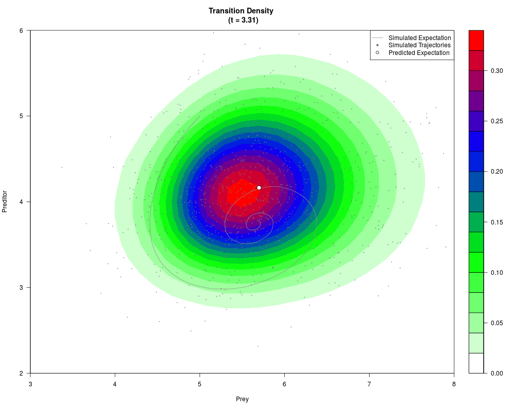
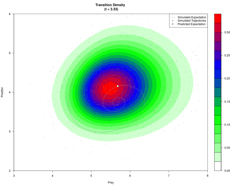
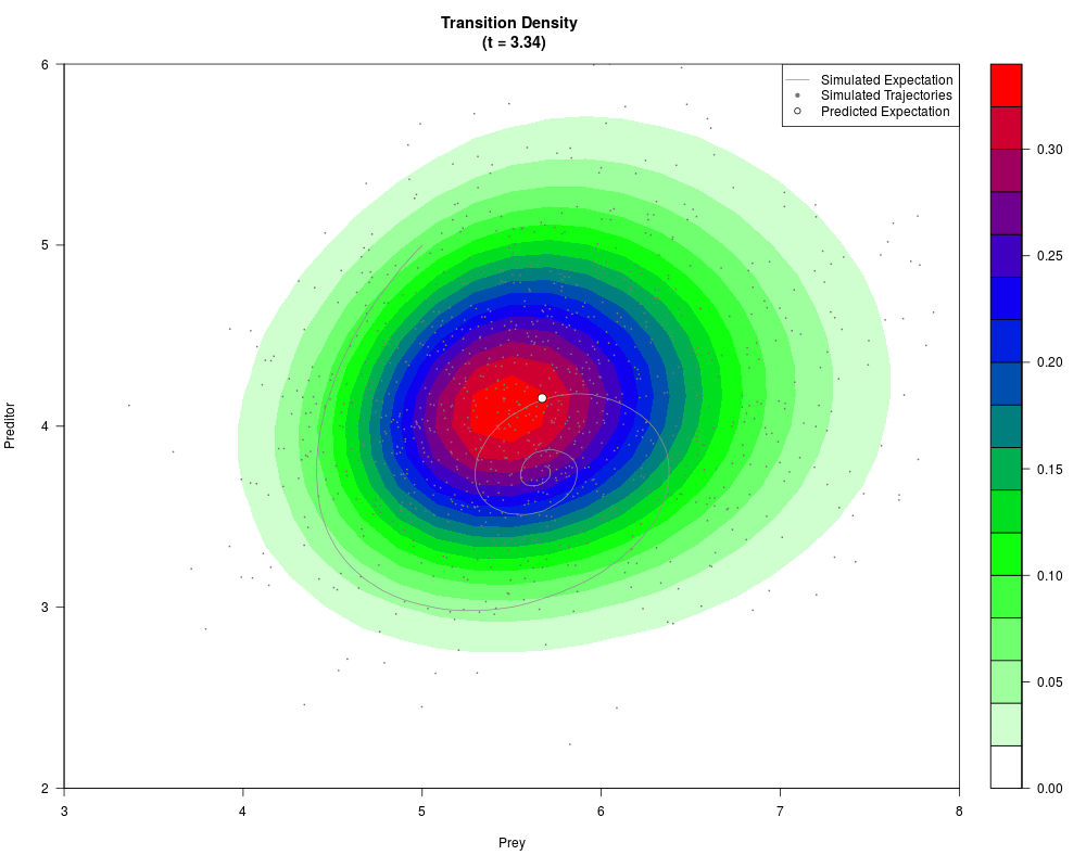
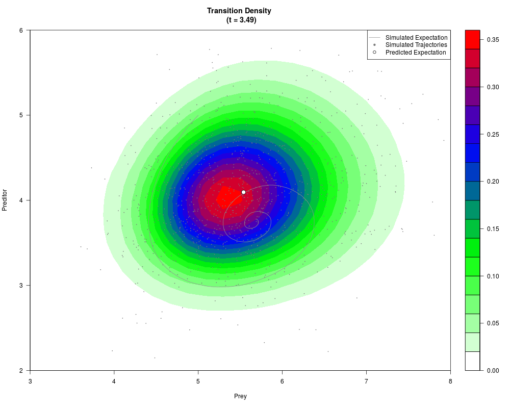
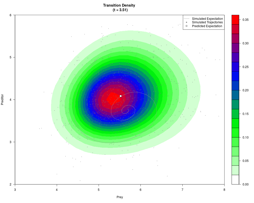
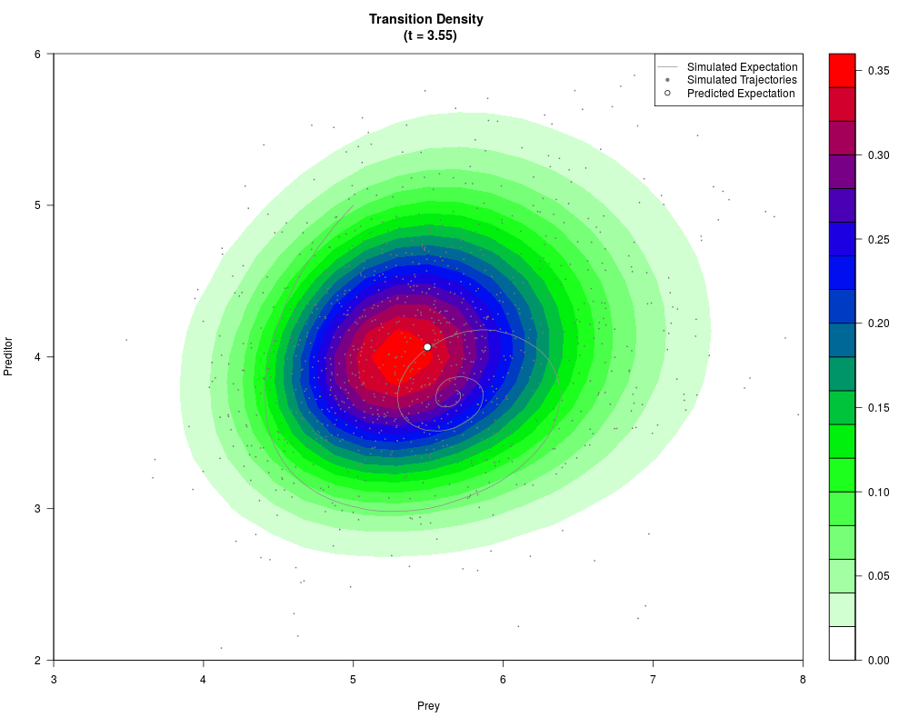
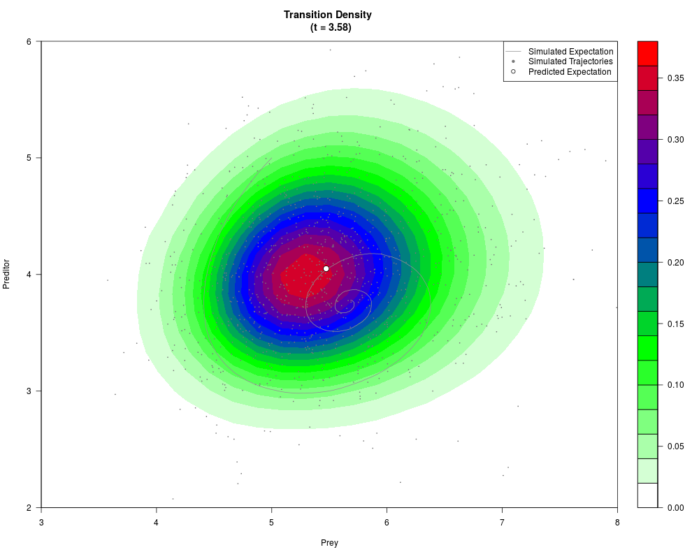
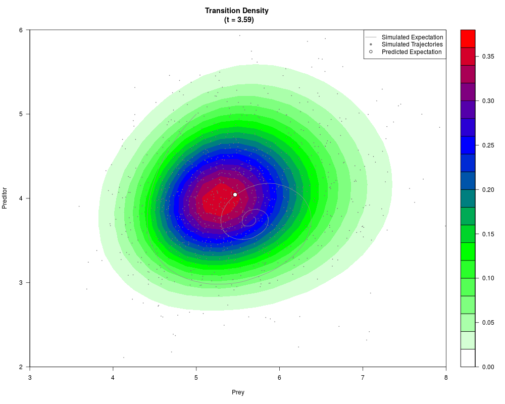
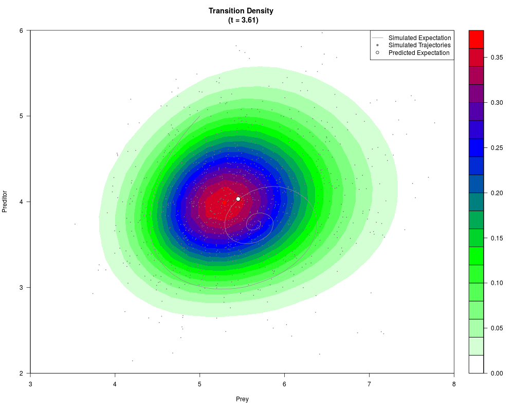
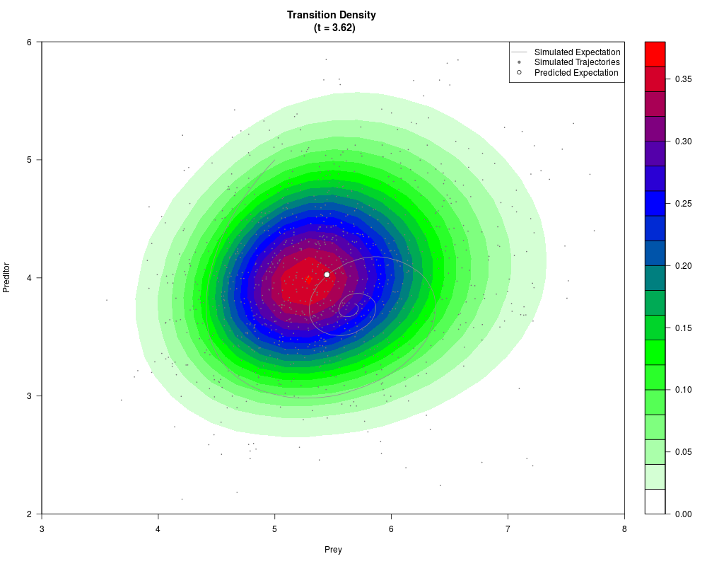
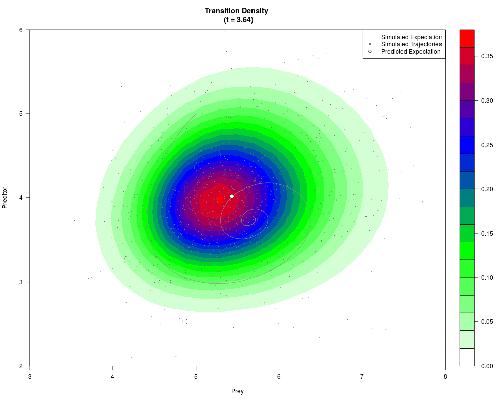
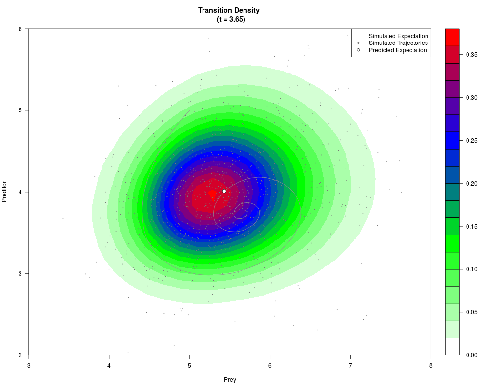
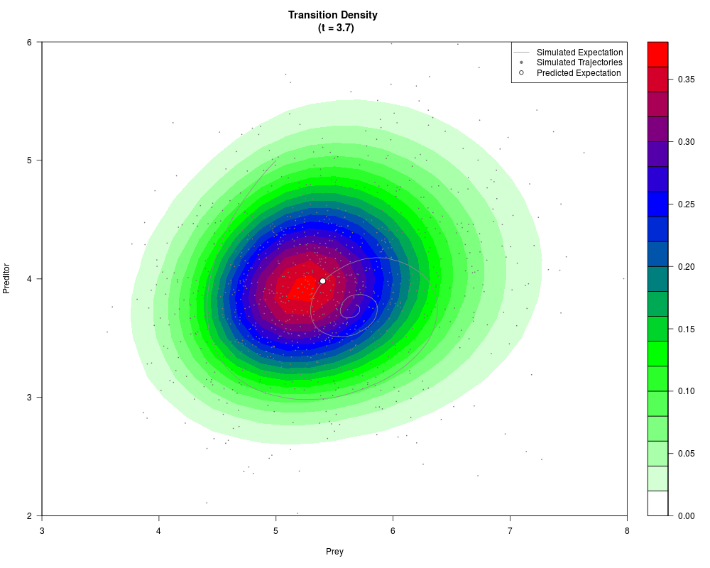
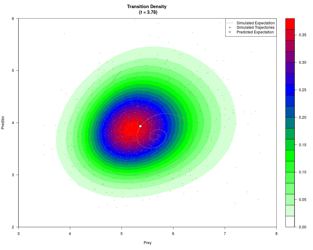
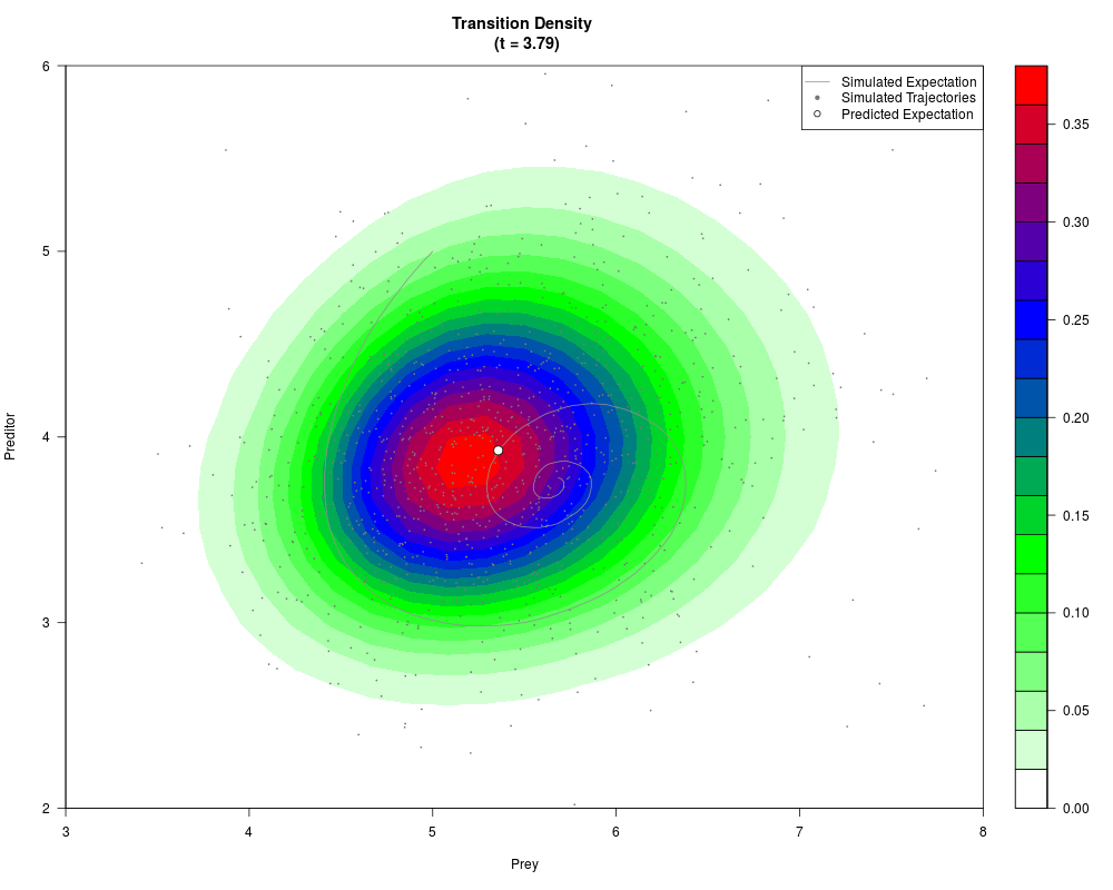
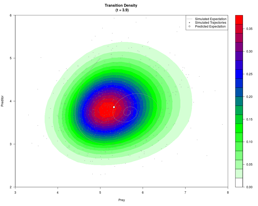
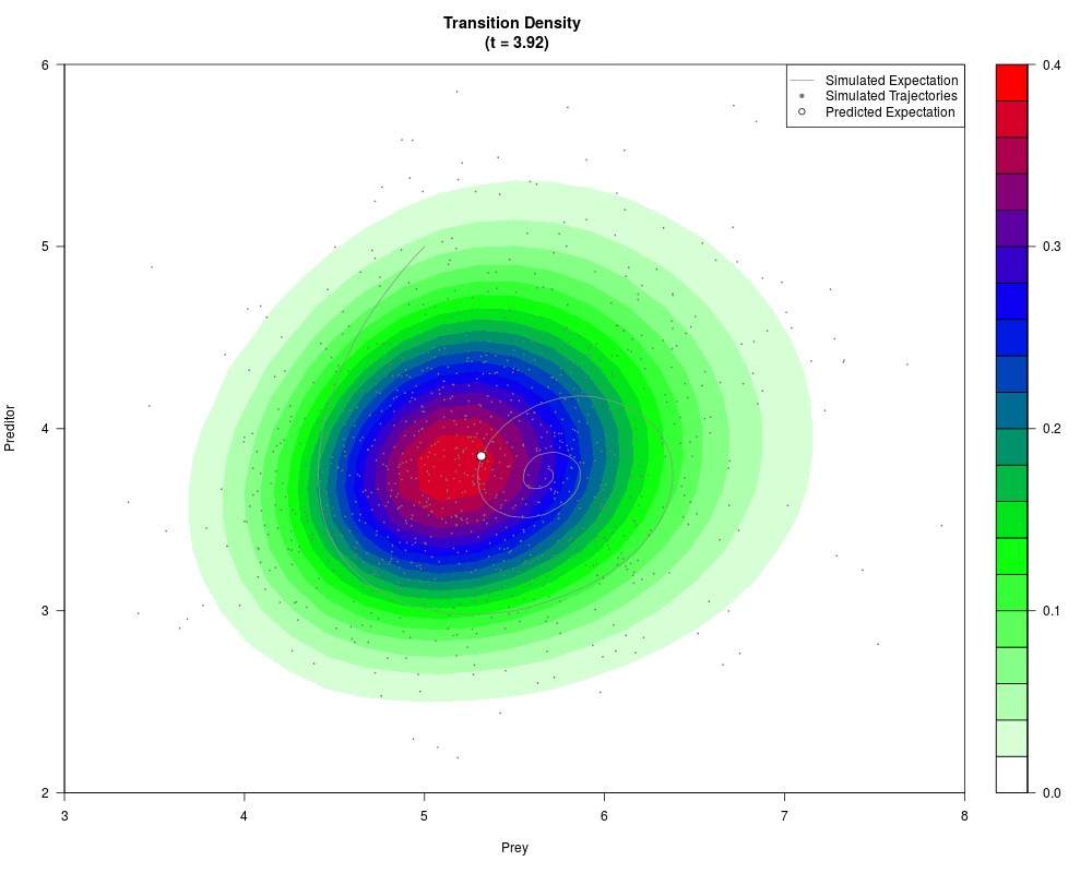
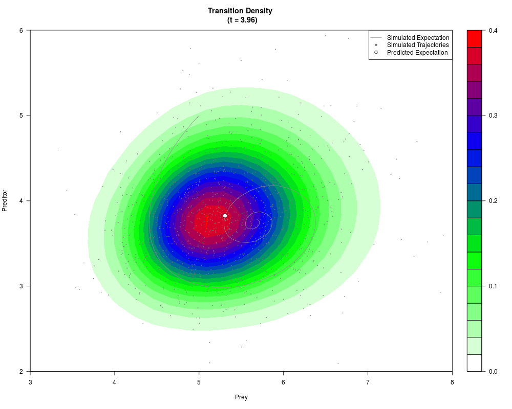
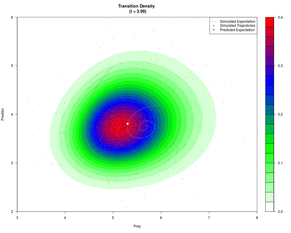
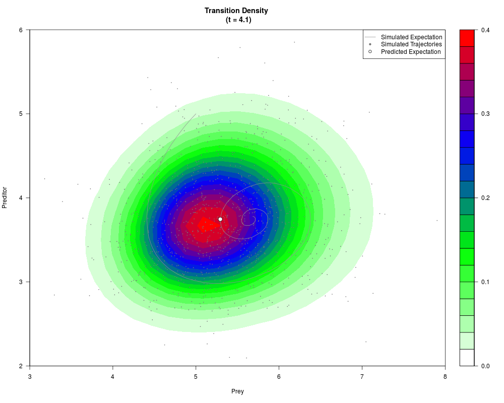
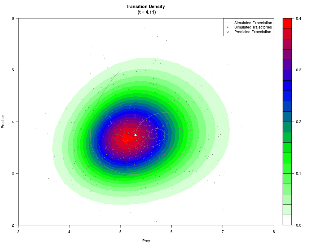
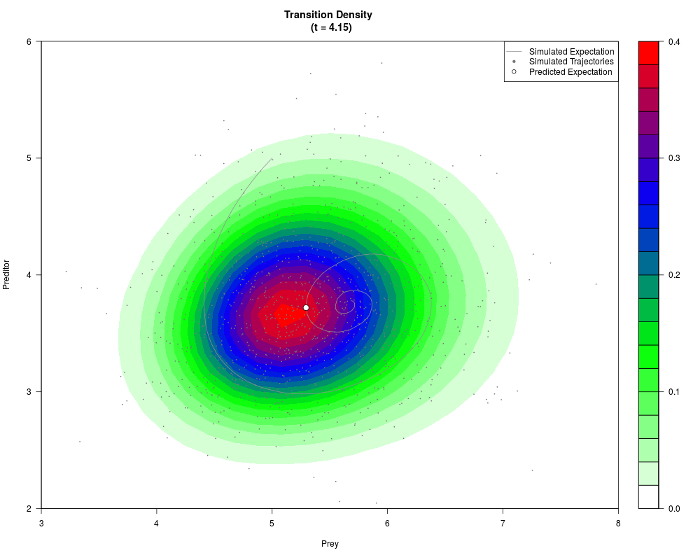
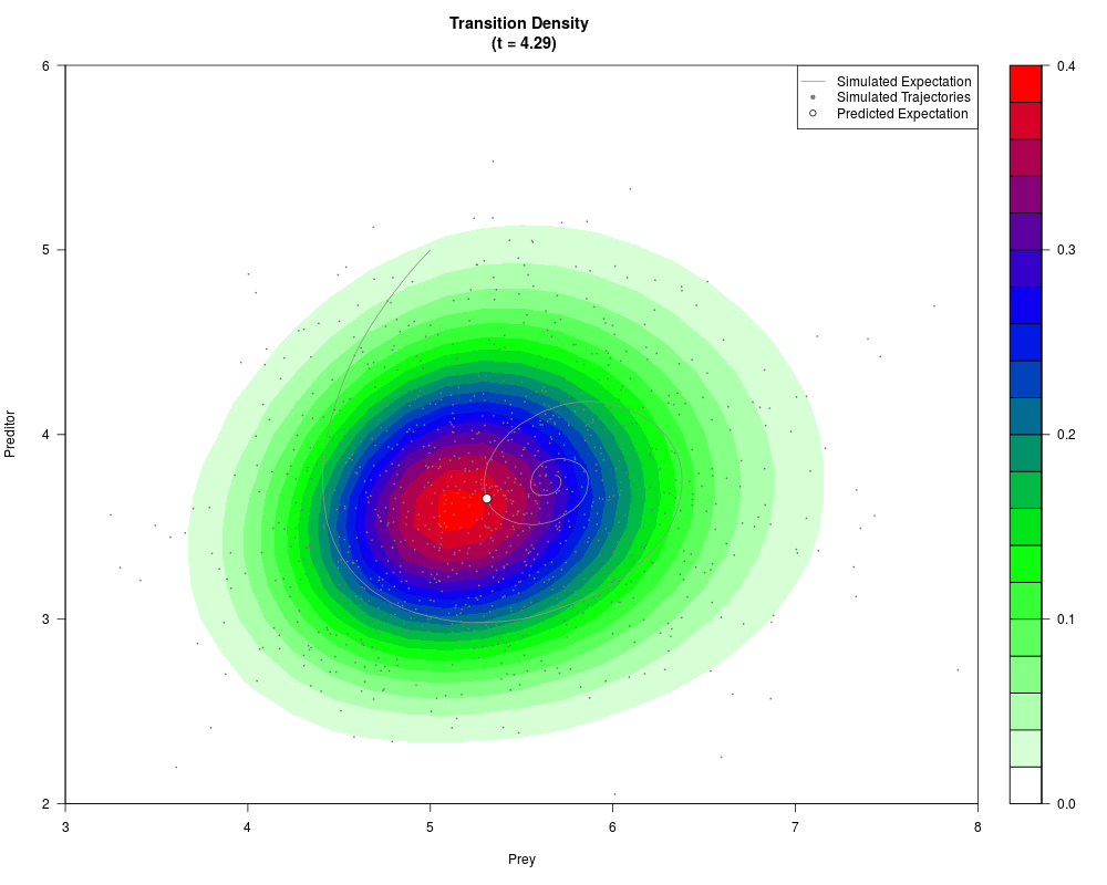
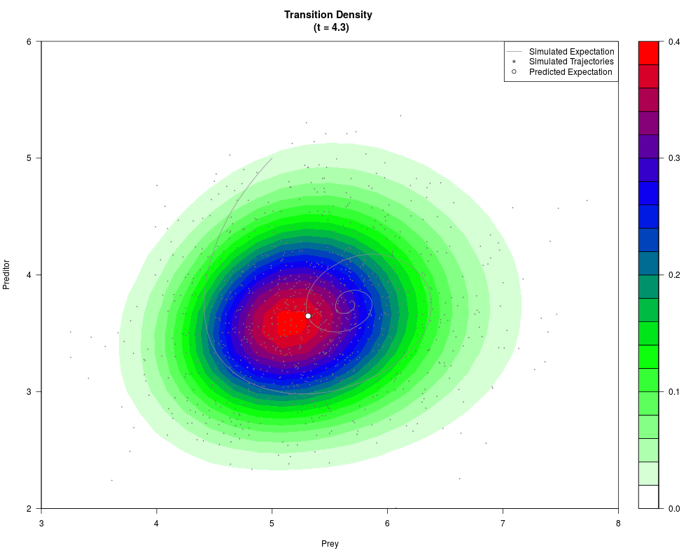
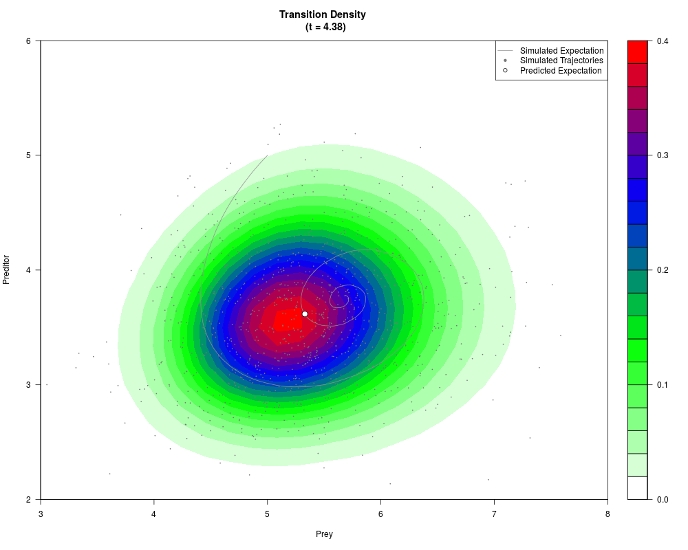
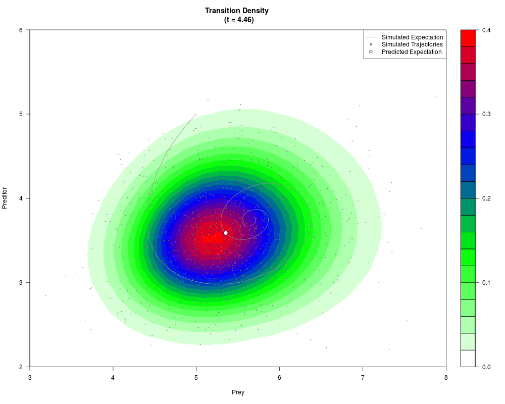
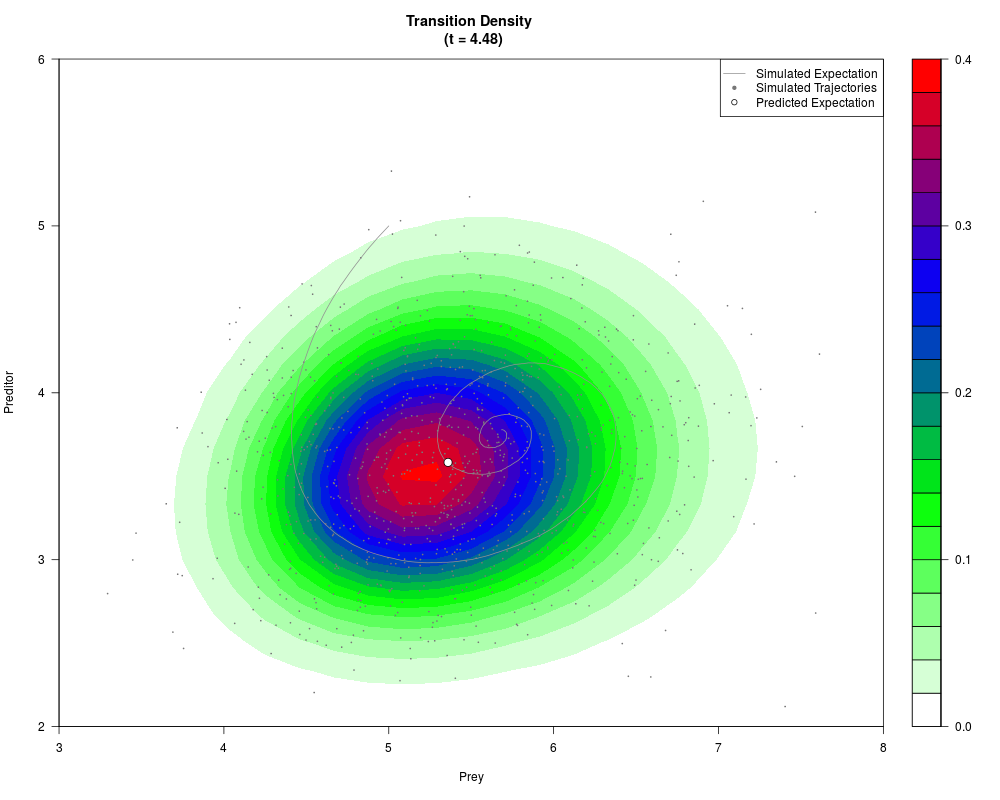
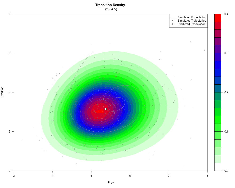
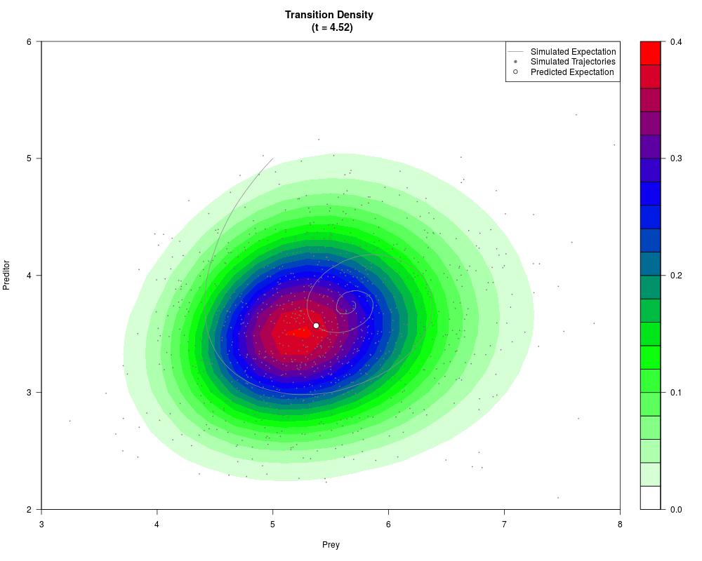
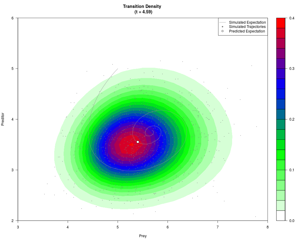
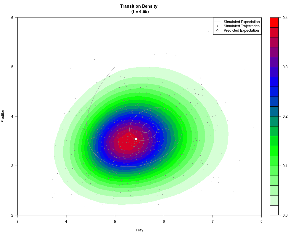
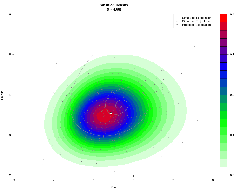
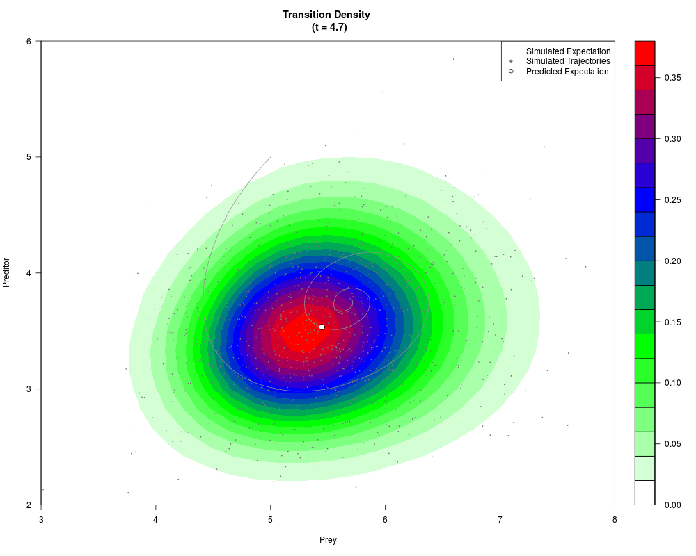
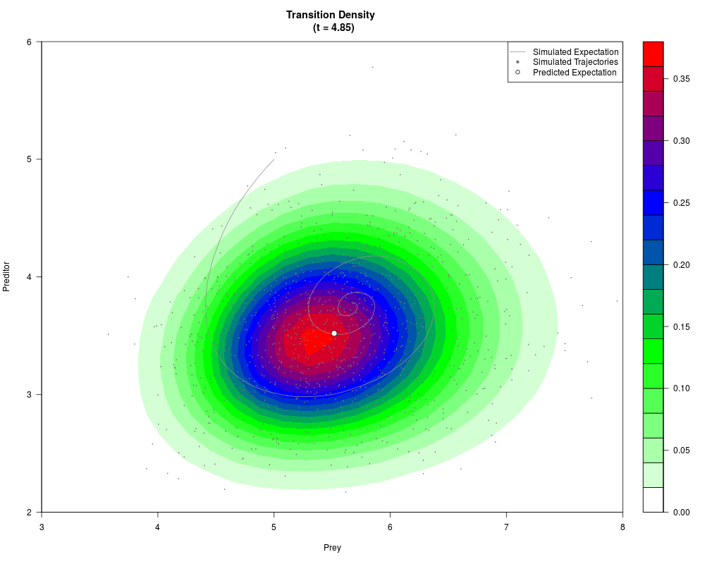
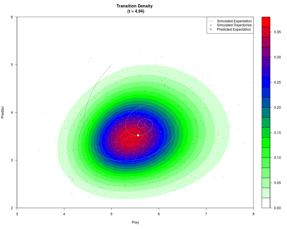
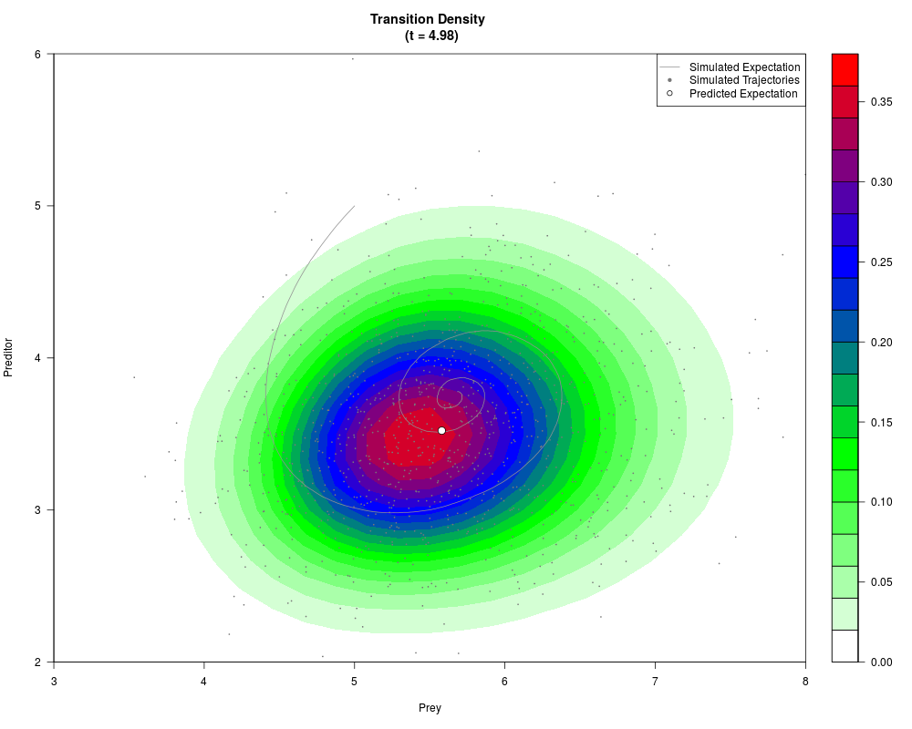
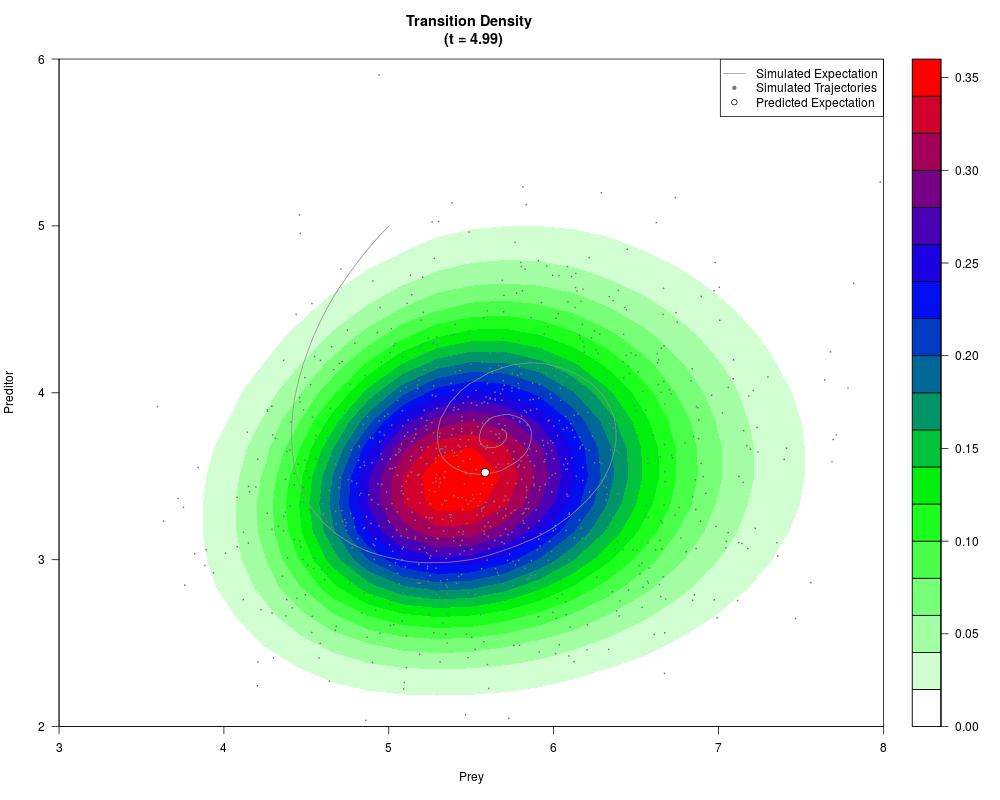
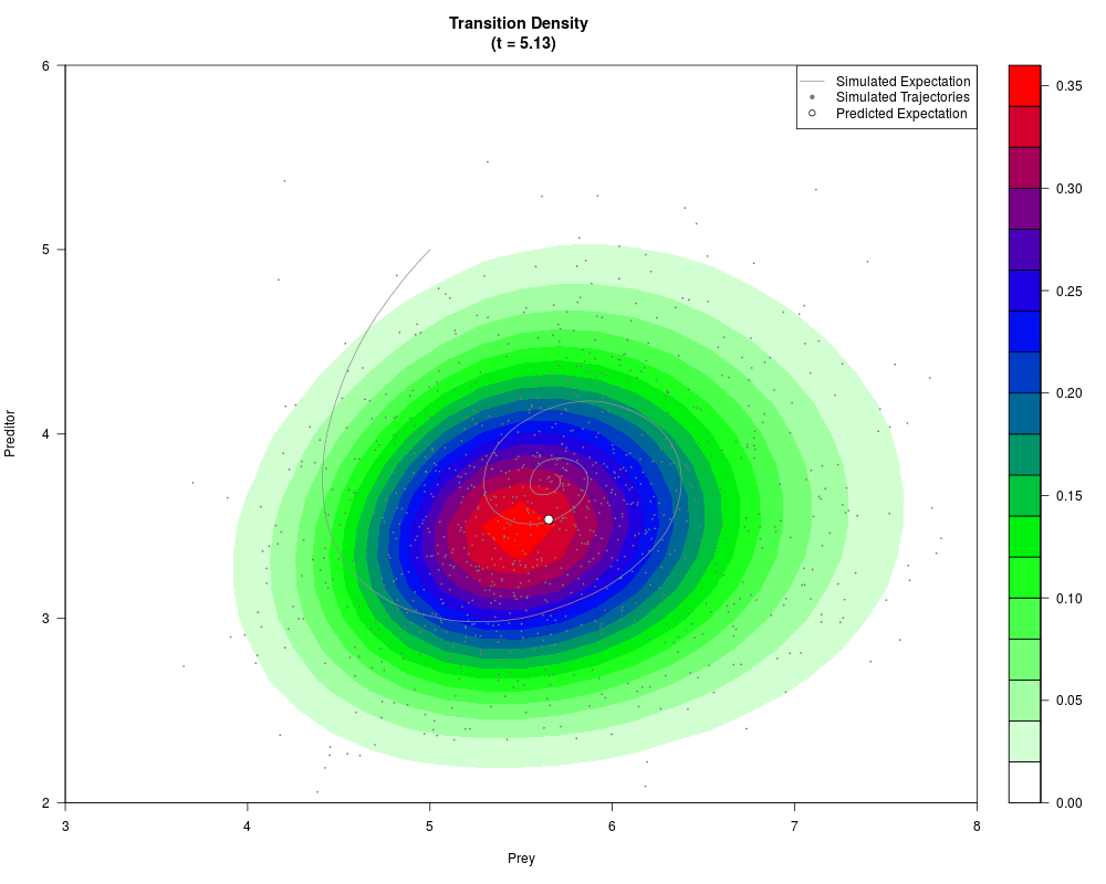
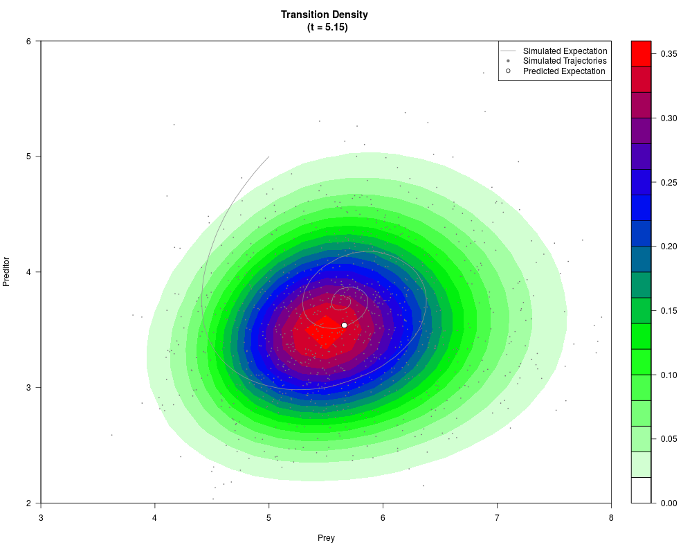
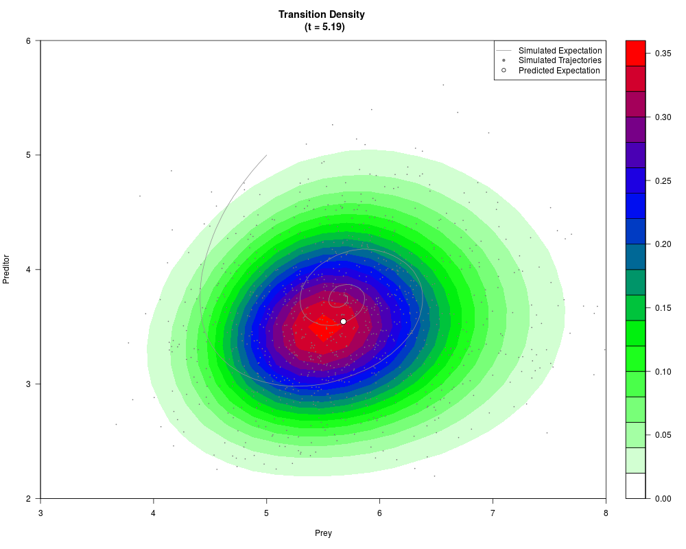
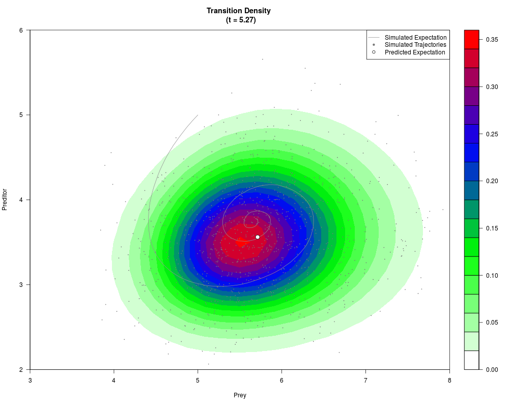
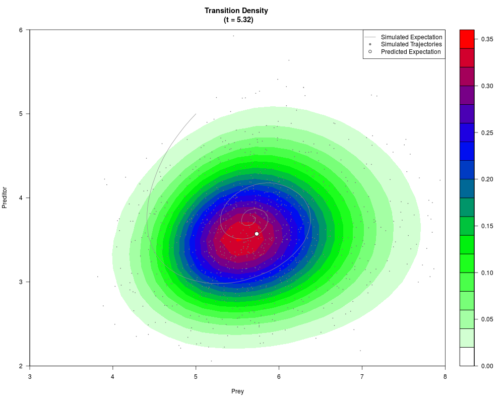
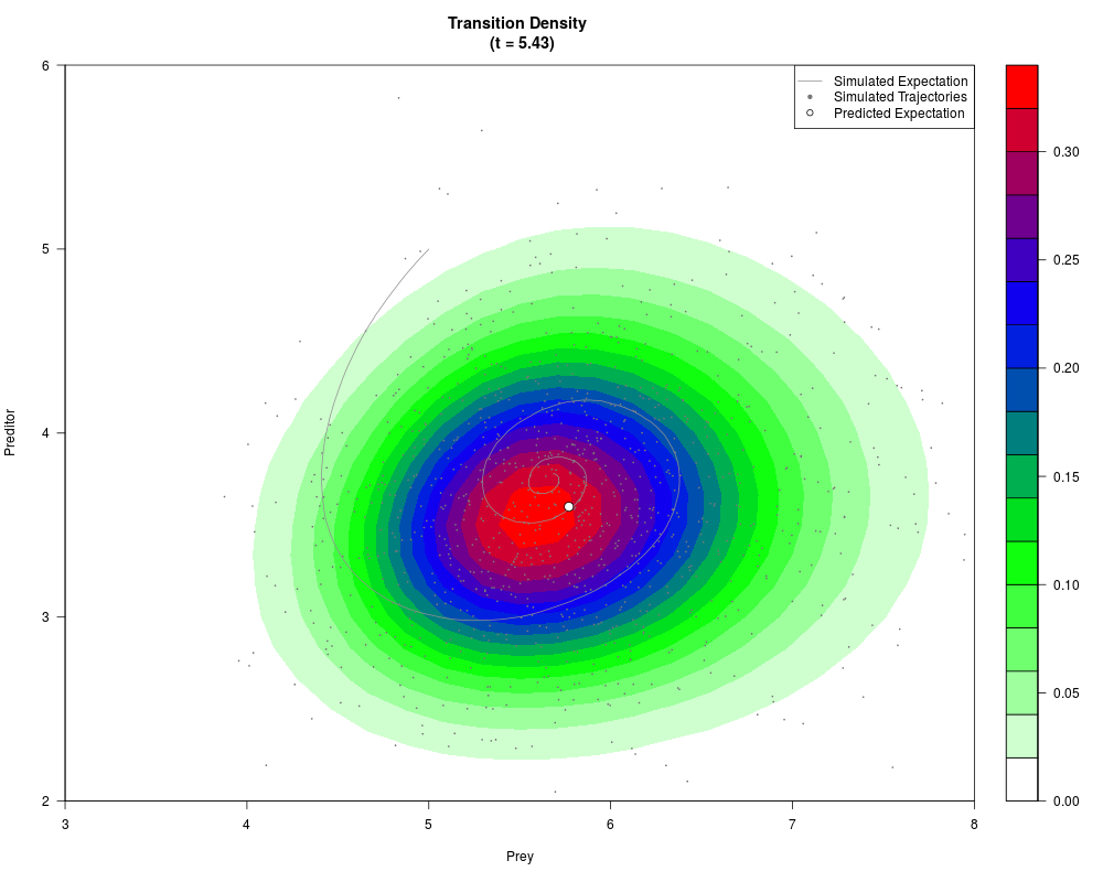
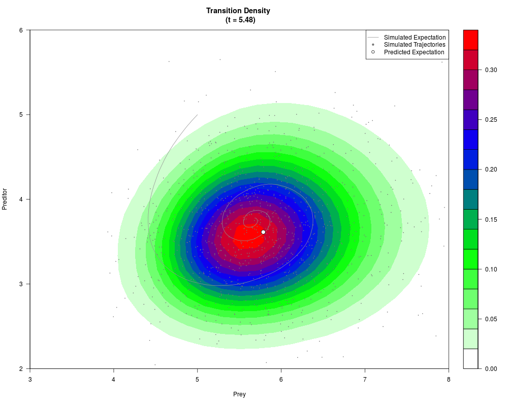
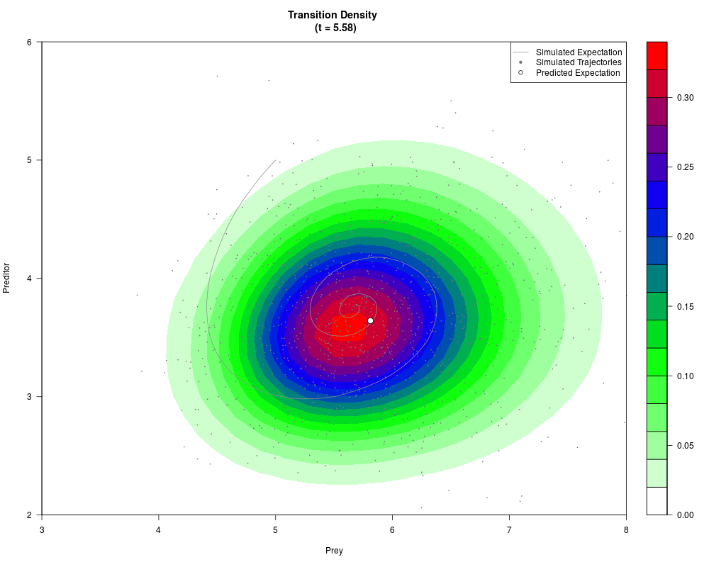
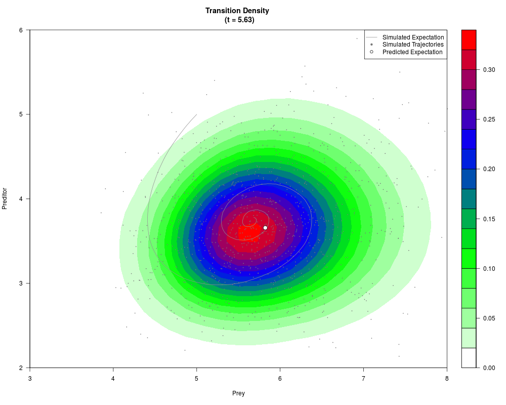
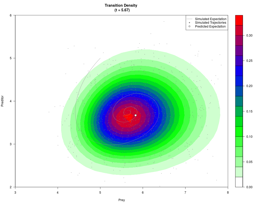
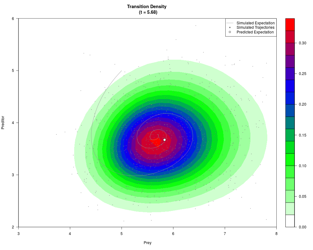
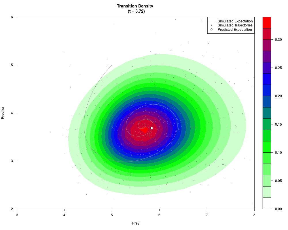
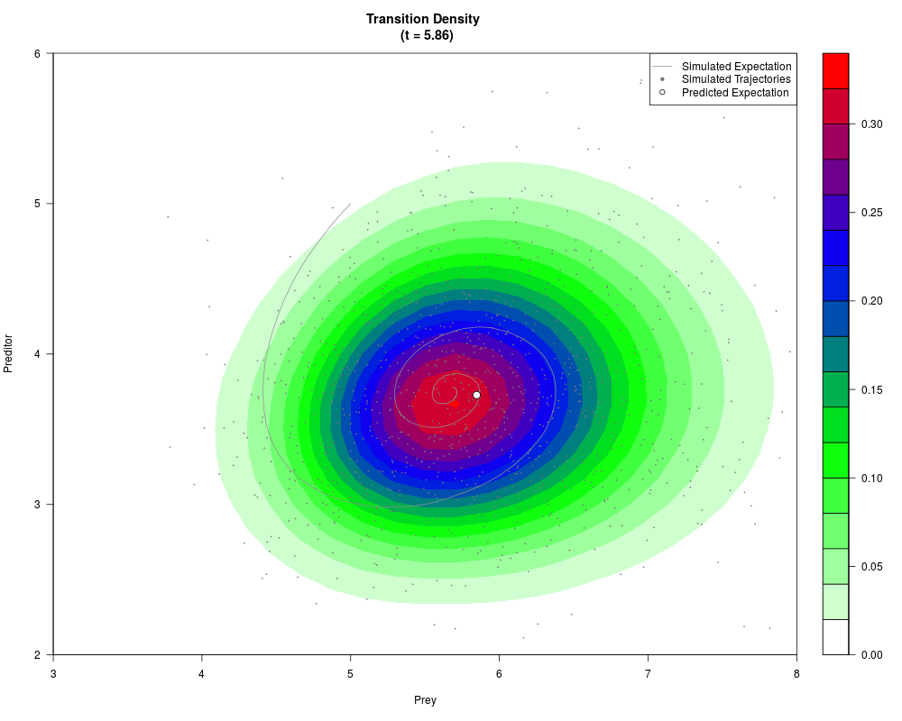
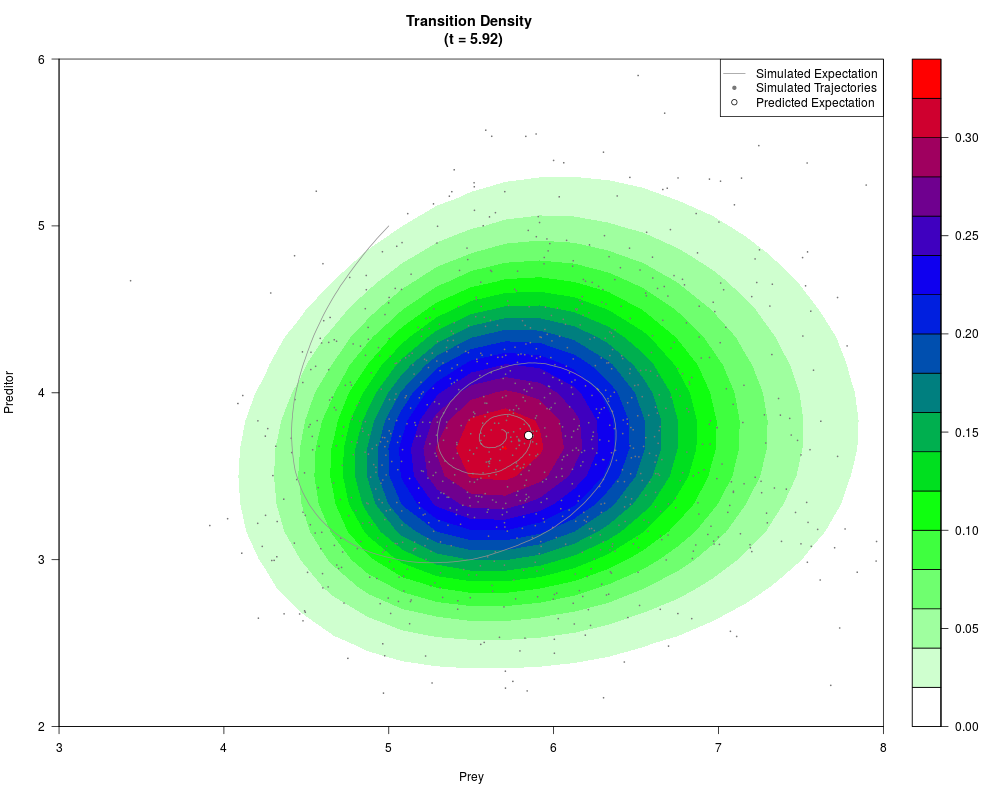
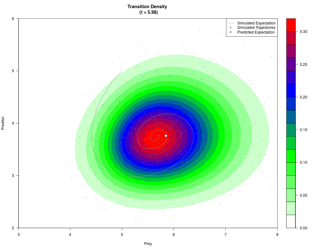
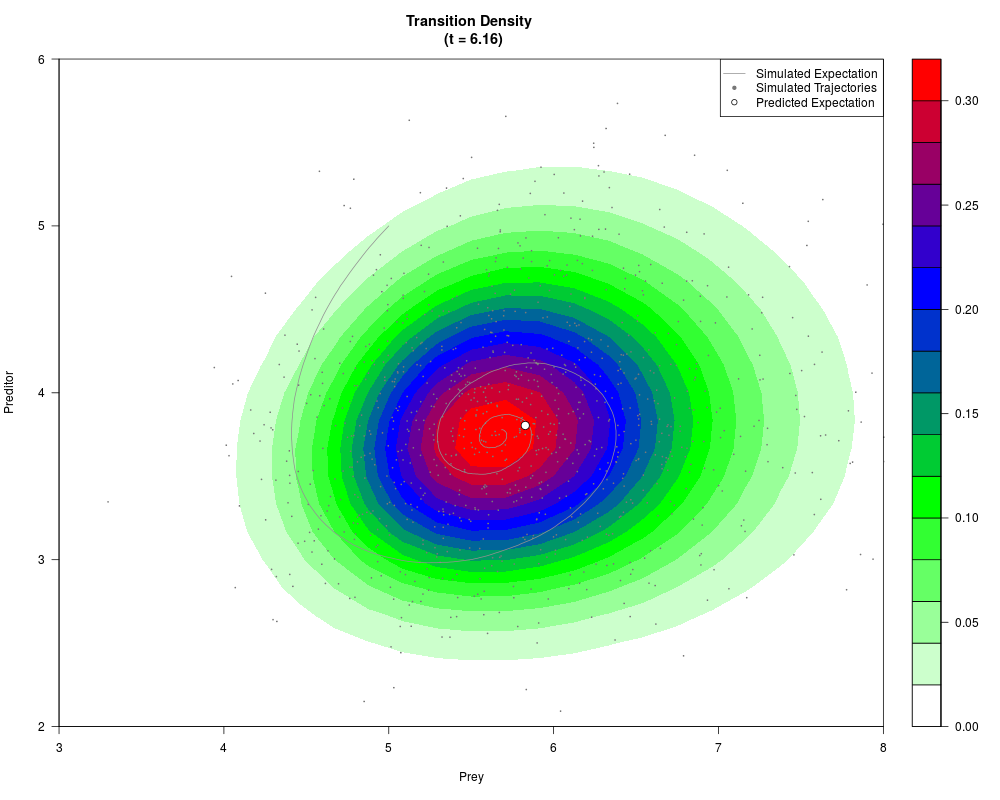
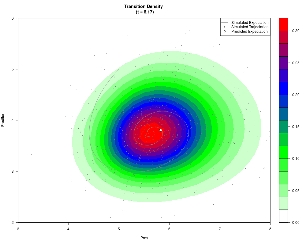
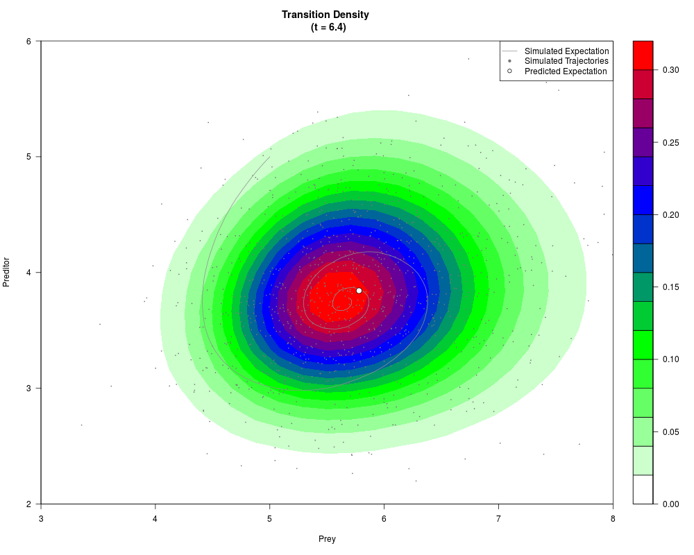
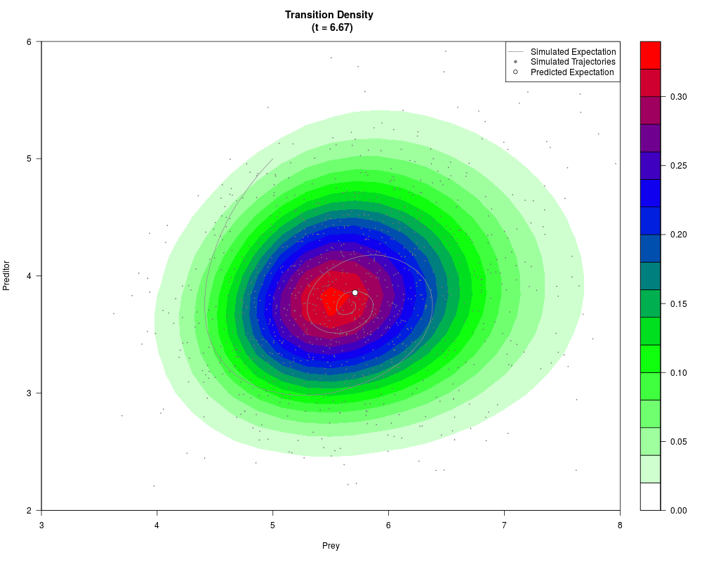
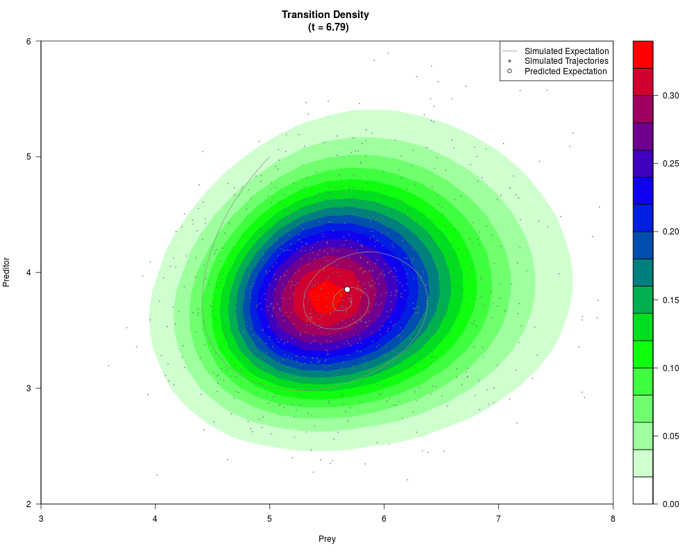
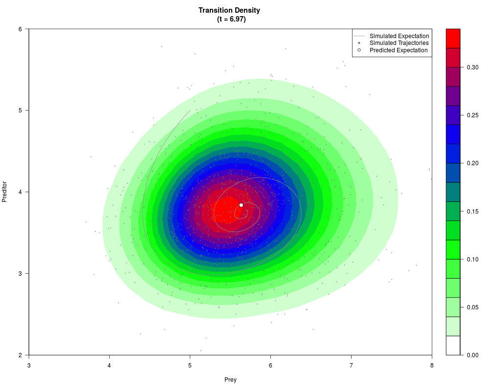
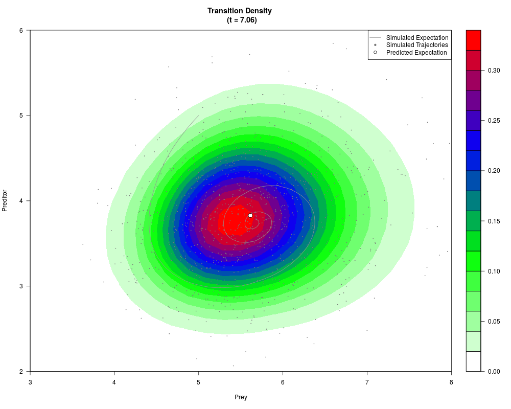
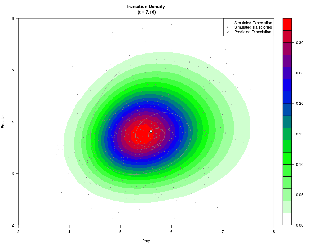
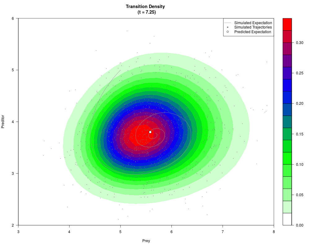
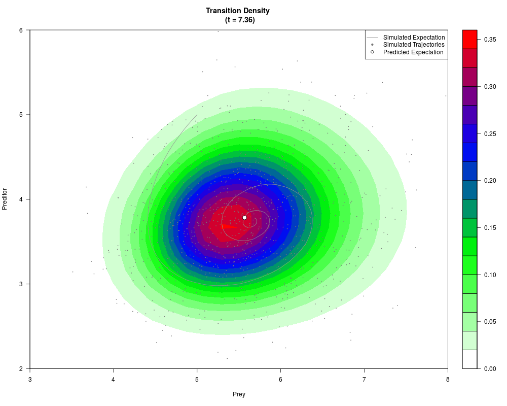
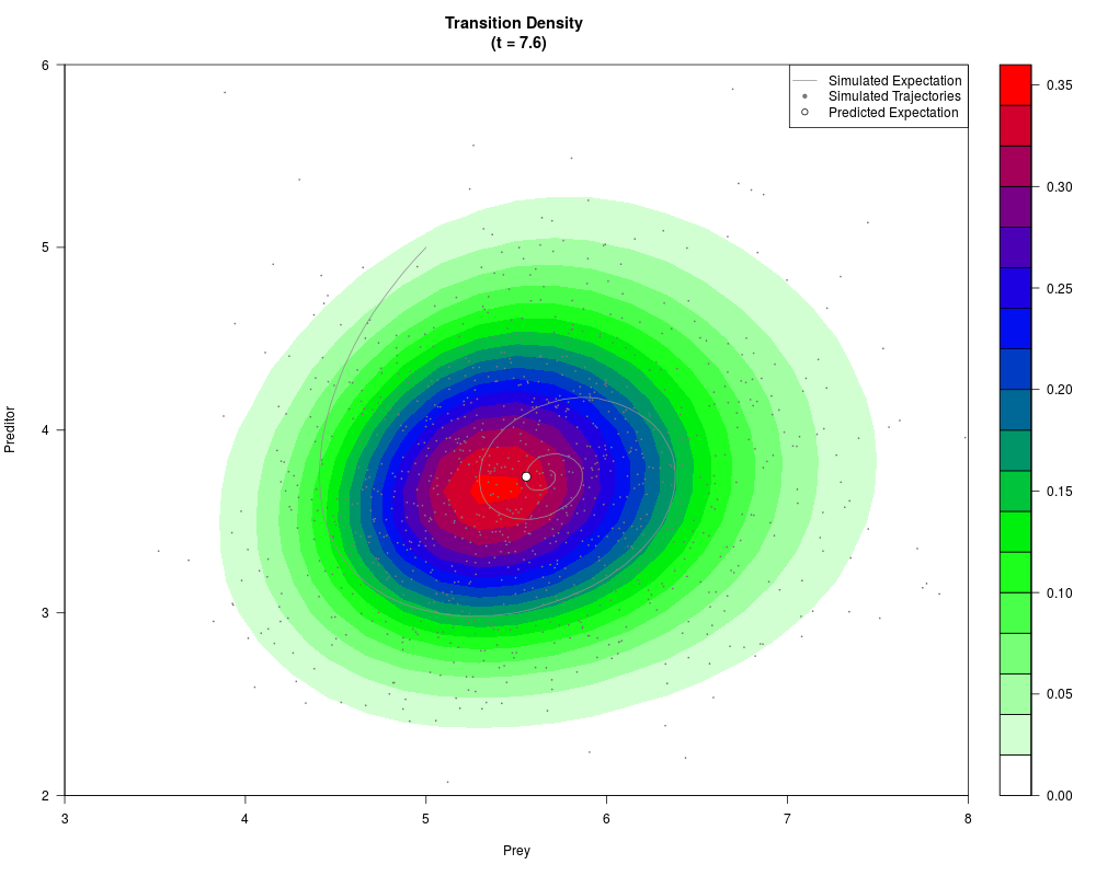
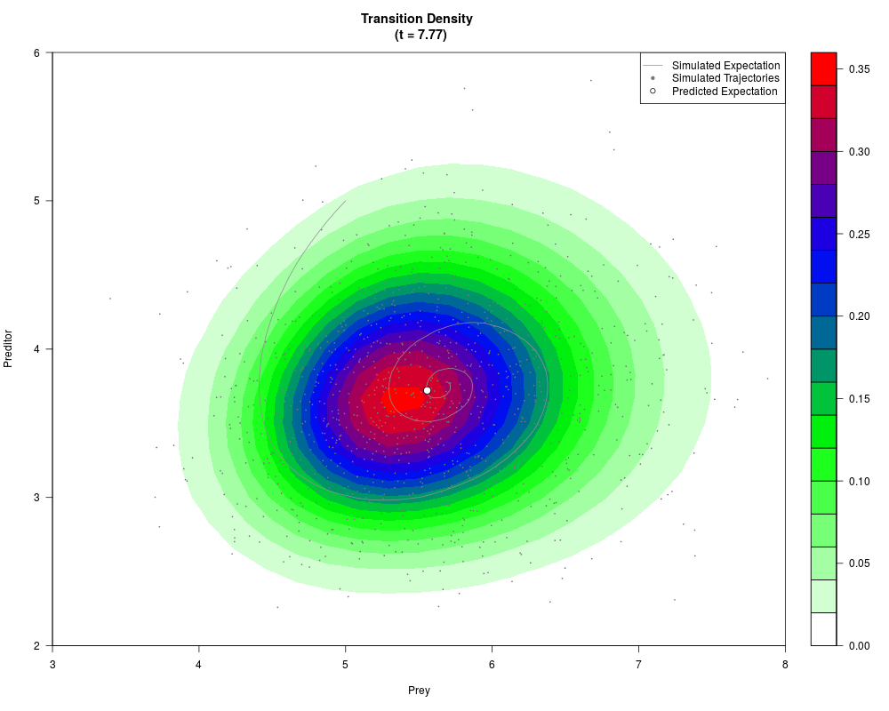
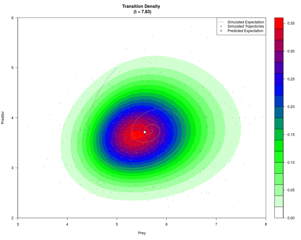
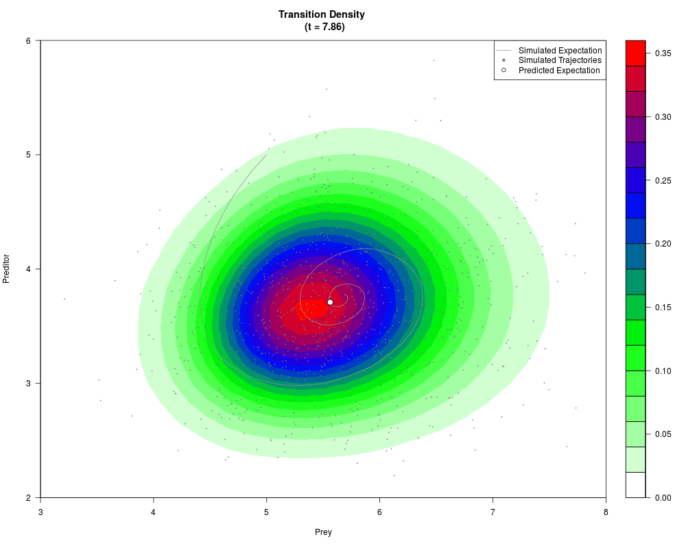
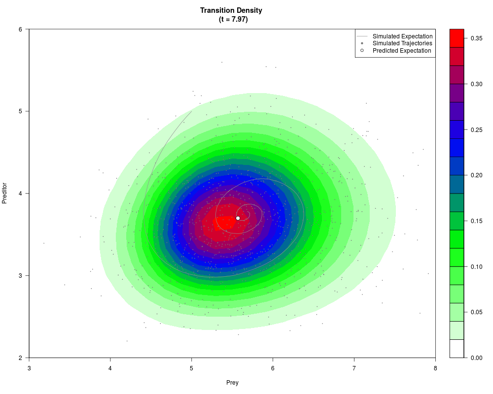
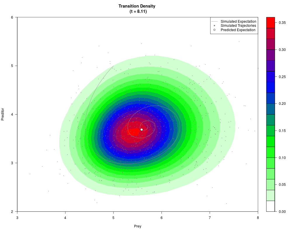
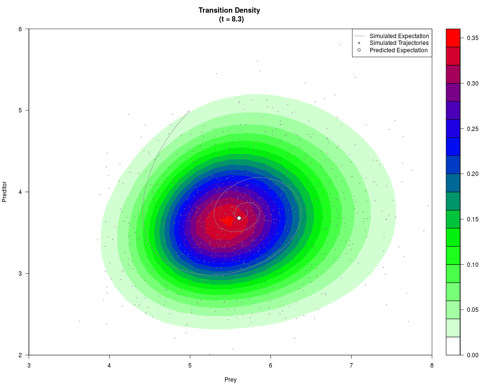
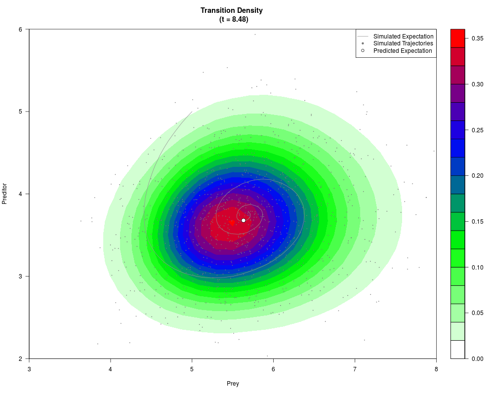
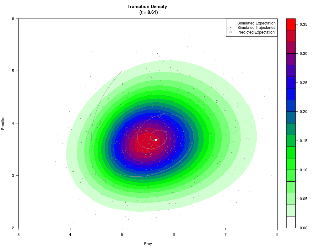
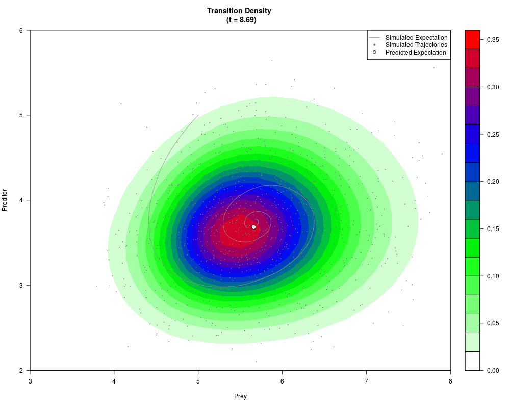
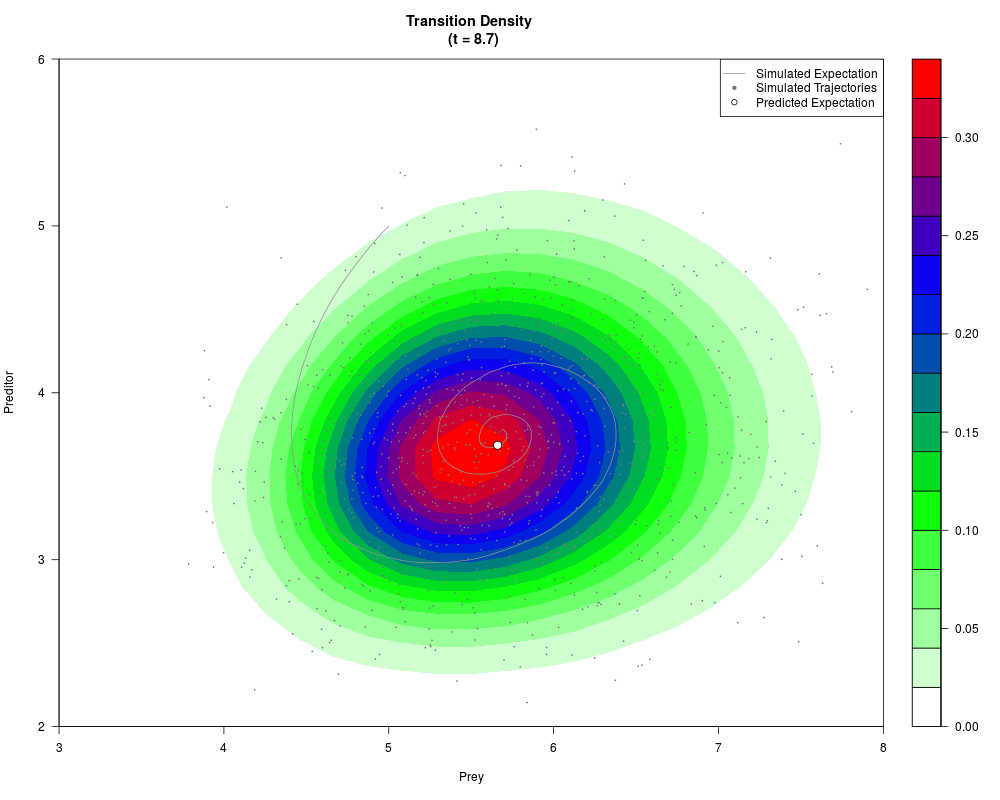
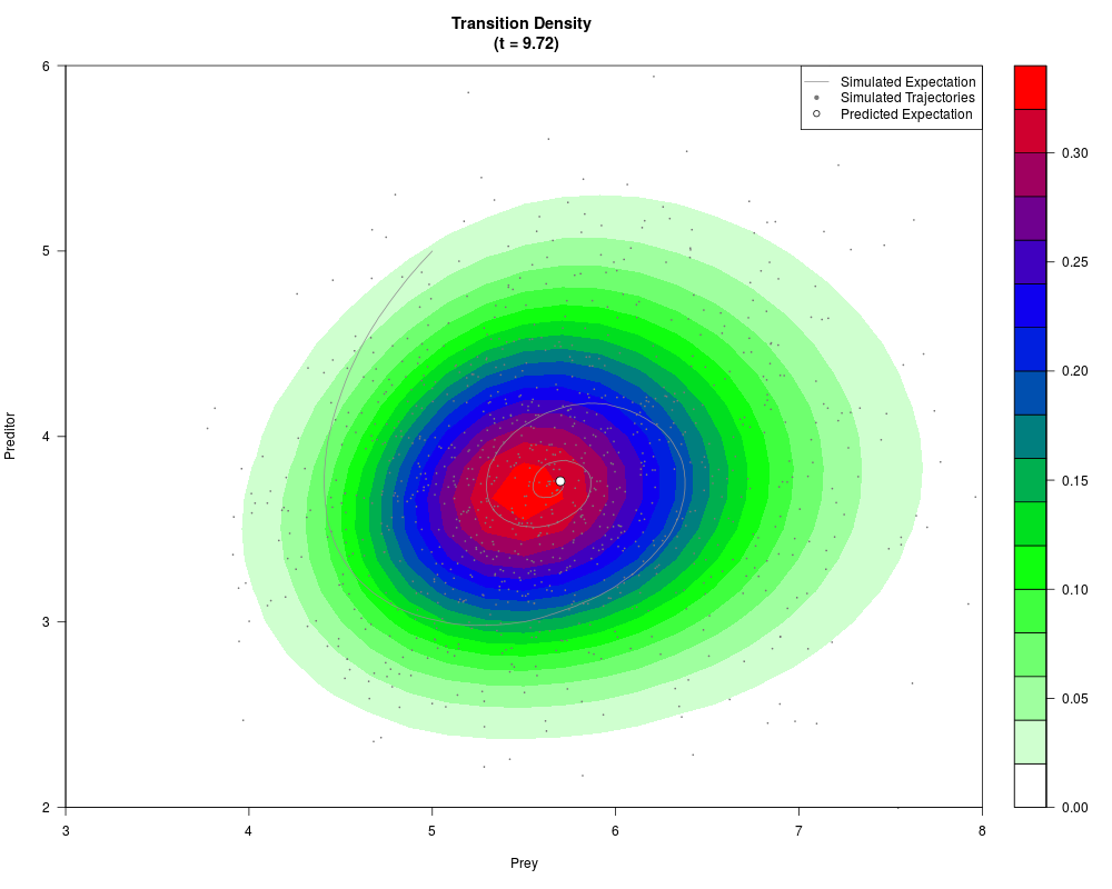
# Generate the transition density of a stochastic perturbed Lotka-Volterra
# preditor-prey model, with state-dependent volatility:
# dX = (1.5X-0.4*X*Y)dt          +sqrt(0.05*X)dWt
# dY = (-1.5Y+0.4*X*Y-0.2*Y^2)dt +sqrt(0.10*Y)dBt
#-------------------------------------------------------------------------------

# Remove any existing coefficients
GQD.remove()

# Define the X dimesnion coefficients
a10 = function(t){1.5}
a11 = function(t){-0.4}
c10 = function(t){0.05}

# Define the Y dimension coefficients
b01 = function(t){-1.5}
b11 = function(t){0.4}
b02 = function(t){-0.2}
f01 = function(t){0.1}

# Approximate the transition density
res = BiGQD.density(5,5,seq(3,8,length=25),seq(2,6,length=25),0,10,1/100)


#------------------------------------------------------------------------------
# Visuallize the density
#------------------------------------------------------------------------------

par(ask=FALSE)
# Load simulated trajectory of the joint expectation:
data(SDEsim3)
attach(SDEsim3)

# We will simulate some trajectories (crudely) as well:
N=1000; delt= 1/100  # 1000 trajectories
X1=rep(5,N)          # Initial values for each trajectory
X2=rep(5,N)

for(i in 1:1001)
{
  # Applly Euler-Murayama scheme to the LV-model
  X1=pmax(X1+(a10(d)*X1+a11(d)*X1*X2)*delt+sqrt(c10(d)*X1)*rnorm(N,sd=sqrt(delt)),0)
  X2=pmax(X2+(b01(d)*X2+b11(d)*X1*X2+b02(d)*X2^2)*delt+sqrt(f01(d)*X2)*rnorm(N,sd=sqrt(delt)),0)

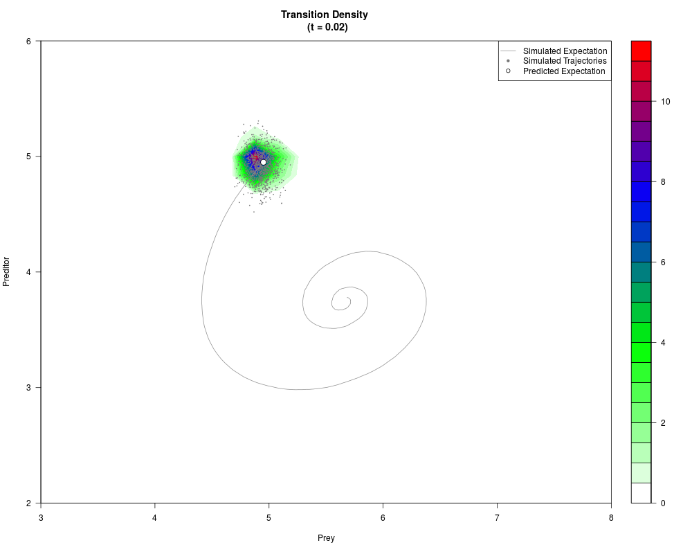
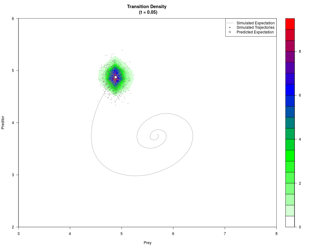
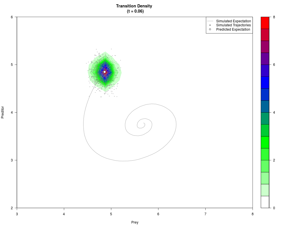
  # Now illustrate the density:
  filled.contour(res$Xt,res$Yt,res$density[,,i],
  main=paste0('Transition Density \n (t = ',res$time[i],')'),
  color.palette=colorRampPalette(c('white','green','blue','red'))
  ,xlab='Prey',ylab='Preditor',plot.axes=
   {
     # Add simulated trajectories
     points(X2~X1,pch=20,col='grey47',cex=0.01)
     # Add trajectory of simulated expectation
     lines(my~mx,col='grey57')
     # Show the predicted expectation from BiGQD.density()
     points(res$cumulants[5,i]~res$cumulants[1,i],bg='white',pch=21,cex=1.5)
     axis(1);axis(2);
     # Add a legend
     legend('topright',lty=c('solid',NA,NA),col=c('grey57','grey47','black'),
             pch=c(NA,20,21),legend=c('Simulated Expectation','Simulated Trajectories'
             ,'Predicted Expectation'))
   })
}

#===============================================================================

Results

R version 3.3.1 (2016-06-21) -- "Bug in Your Hair"
Copyright (C) 2016 The R Foundation for Statistical Computing
Platform: x86_64-pc-linux-gnu (64-bit)

R is free software and comes with ABSOLUTELY NO WARRANTY.
You are welcome to redistribute it under certain conditions.
Type 'license()' or 'licence()' for distribution details.

R is a collaborative project with many contributors.
Type 'contributors()' for more information and
'citation()' on how to cite R or R packages in publications.

Type 'demo()' for some demos, 'help()' for on-line help, or
'help.start()' for an HTML browser interface to help.
Type 'q()' to quit R.

> library(DiffusionRgqd)
> png(filename="/home/ddbj/snapshot/RGM3/R_CC/result/DiffusionRgqd/BiGQD.density.Rd_%03d_medium.png", width=480, height=480)
> ### Name: BiGQD.density
> ### Title: Generate the Transition Density of a Bivariate Generalized
> ###   Quadratic Diffusion Model (2D GQD).
> ### Aliases: BiGQD.density
> ### Keywords: transition density bivariate saddlepoint bivariate Edgeworth
> ###   moments cumulants
> 
> ### ** Examples
> 
> ## No test: 
> #===============================================================================
> # Generate the transition density of a stochastic perturbed Lotka-Volterra
> # preditor-prey model, with state-dependent volatility:
> # dX = (1.5X-0.4*X*Y)dt          +sqrt(0.05*X)dWt
> # dY = (-1.5Y+0.4*X*Y-0.2*Y^2)dt +sqrt(0.10*Y)dBt
> #-------------------------------------------------------------------------------
> 
> # Remove any existing coefficients
> GQD.remove()
[1] "Removed :  NA "
> 
> # Define the X dimesnion coefficients
> a10 = function(t){1.5}
> a11 = function(t){-0.4}
> c10 = function(t){0.05}
> 
> # Define the Y dimension coefficients
> b01 = function(t){-1.5}
> b11 = function(t){0.4}
> b02 = function(t){-0.2}
> f01 = function(t){0.1}
> 
> # Approximate the transition density
> res = BiGQD.density(5,5,seq(3,8,length=25),seq(2,6,length=25),0,10,1/100)
                                                                 
 ================================================================
                   GENERALIZED QUADRATIC DIFFUSON                
 ================================================================
 _____________________ Drift Coefficients _______________________
 a10 : 1.5                                                       
 a11 : -0.4                                                      
 ...   ...   ...   ...   ...   ...   ...   ...   ...   ...   ... 
 b01 : -1.5                                                      
 b02 : -0.2                                                      
 b11 : 0.4                                                       
 ___________________ Diffusion Coefficients _____________________
 c10 : 0.05                                                      
 ...   ...   ...   ...   ...   ...   ...   ...   ...   ...   ... 
 ...   ...   ...   ...   ...   ...   ...   ...   ...   ...   ... 
 ...   ...   ...   ...   ...   ...   ...   ...   ...   ...   ... 
 f01 : 0.1                                                       
=================================================================
> 
> 
> #------------------------------------------------------------------------------
> # Visuallize the density
> #------------------------------------------------------------------------------
> 
> par(ask=FALSE)
> # Load simulated trajectory of the joint expectation:
> data(SDEsim3)
> attach(SDEsim3)
> 
> # We will simulate some trajectories (crudely) as well:
> N=1000; delt= 1/100  # 1000 trajectories
> X1=rep(5,N)          # Initial values for each trajectory
> X2=rep(5,N)
> 
> for(i in 1:1001)
+ {
+   # Applly Euler-Murayama scheme to the LV-model
+   X1=pmax(X1+(a10(d)*X1+a11(d)*X1*X2)*delt+sqrt(c10(d)*X1)*rnorm(N,sd=sqrt(delt)),0)
+   X2=pmax(X2+(b01(d)*X2+b11(d)*X1*X2+b02(d)*X2^2)*delt+sqrt(f01(d)*X2)*rnorm(N,sd=sqrt(delt)),0)
+ 
+   # Now illustrate the density:
+   filled.contour(res$Xt,res$Yt,res$density[,,i],
+   main=paste0('Transition Density \n (t = ',res$time[i],')'),
+   color.palette=colorRampPalette(c('white','green','blue','red'))
+   ,xlab='Prey',ylab='Preditor',plot.axes=
+    {
+      # Add simulated trajectories
+      points(X2~X1,pch=20,col='grey47',cex=0.01)
+      # Add trajectory of simulated expectation
+      lines(my~mx,col='grey57')
+      # Show the predicted expectation from BiGQD.density()
+      points(res$cumulants[5,i]~res$cumulants[1,i],bg='white',pch=21,cex=1.5)
+      axis(1);axis(2);
+      # Add a legend
+      legend('topright',lty=c('solid',NA,NA),col=c('grey57','grey47','black'),
+              pch=c(NA,20,21),legend=c('Simulated Expectation','Simulated Trajectories'
+              ,'Predicted Expectation'))
+    })
+ }
> 
> #===============================================================================
> ## End(No test)
> 
> 
> 
> 
> 
> 
> dev.off()
null device 
          1 
>