R Graphical Manual

Browse All

Last data update: 2014.03.03

R: MCMC Inference on Bivariate Generalized Quadratic Diffusions...

BiGQD.mcmc

R Documentation

MCMC Inference on Bivariate Generalized Quadratic Diffusions (2D GQDs).

Description

BiGQD.mcmc() uses parametrised coefficients (provided by the user as R-functions) to construct a C++ program in real time that allows the user to perform Bayesian inference on the resulting diffusion model. Given a set of starting parameters and other input parameters, a MCMC chain is returned for further analysis. BiGQD.density generates approximate transitional densities for a class of bivariate diffusion processes with SDE:

where

and

Usage

BiGQD.mcmc(X, time, mesh=10, theta, sds, updates, burns=min(round(updates/2),25000),
           RK.order=4, exclude=NULL, plot.chain=TRUE, Tag=NA, Dtype='Saddlepoint',
           recycle=FALSE, rtf=runif(2), wrt=FALSE, print.output=TRUE)

Arguments

`X`	A matrix containing rows of data points to be modelled. Although observations are allowed to be non-equidistant, observations in both dimensions are assumed to occur at the same time epochs (i.e. `time` gives the time signature for both dimensions).
`time`	A vector containing the time epochs at which observations were made.
`mesh`	The number of mesh points in the time discretization.
`theta`	The parameter vector of the process. theta are taken as the starting values of the MCMC chain and gives the dimension of the parameter vector used to calculate the DIC. Care should be taken to ensure that each element in theta is in fact used within the coefficient-functions, otherwise redundant parameters will be counted in the calculation of the DIC.
`sds`	Proposal distribution standard deviations. That is, for the i-th parameter the proposal distribution is ~ Normal(...,`sds`[i]^2).
`updates`	The number of MCMC updates/iterations to perform (including burn-in).
`burns`	The number of MCMC updates/iterations to burn.
`exclude`	Vector indicating which transitions to exclude from the analysis. Default = `NULL`.
`plot.chain`	If = TRUE (default), a trace plot of the MCMC chain will be made along with a trace of the acceptance rate.
`RK.order`	The order of the Runge-Kutta solver used to approximate the trajectories of cumulants. Must be 4 (default) or 10.
`Tag`	`Tag` can be used to name (tag) an MCMC run e.g. `Tag='Run_1'`
`Dtype`	The density approximant to use. Valid types are `"Saddlepoint"` (default), `"Edgeworth"` or `"Normal"`.
`recycle`	Whether or not to recycle the roots calculated for the saddlepoint approximation over succesive updates.
`rtf`	Starting vector for internal use.
`wrt`	If `TRUE` a .cpp file will be written to the current directory. For bug report diagnostics.
`print.output`	If `TRUE` information about the model and algorithm is printed to the console.

Value

`par.matrix`	A matrix containing the MCMC chain on `theta`.
`acceptence.rate`	A vector containing the acceptance rate of the MCMC at every iteration.
`model.info`	A list of variables pertaining to inference calculations.
`model.info$elapsed.time`	The runtime, in h/m/s format,of the MCMC procedure (excluding compile time).
`model.info$time.homogeneous`	‘No’ if the model has time-homogeneous coefficients and ‘Yes’ otherwise.
`model.info$p`	The dimension of `theta`.
`model.info$DIC`	Calculated Deviance Information Criterion.
`model.info$pd`	Effective number of parameters (see `model.info$DIC`).

Syntactical jargon

Synt. [1]: The coefficients of the 2D GQD may be parameterized using the reserved variable theta. For example:

a00 <- function(t){theta[1]*(theta[2]+sin(2*pi*(t-theta[3])))}.

Synt. [2]: Due to syntactical differences between R and C++ special functions have to be used when terms that depend on t. When the function cannot be separated in to terms that contain a single t, the prod(a,b) function must be used. For example:

a00 <- function(t){0.1*(10+0.2*sin(2*pi*t)+0.3*prod(sqrt(t),1+cos(3*pi*t)))}.

Here sqrt(t)*cos(3*pi*t) constitutes the product of two terms that cannot be written i.t.o. a single t. To circumvent this isue, one may use the prod(a,b) function.

Synt. [3]: Similarly, the ^ - operator is not overloaded in C++. Instead the pow(x,p) function may be used to calculate x^p. For example sin(2*pi*t)^3 in:

a00 <- function(t){0.1*(10+0.2*pow(sin(2*pi*t),3))}.

Warning

Warning [1]: The parameter mesh is used to discretize the transition horizons between successive observations. It is thus important to ensure that mesh is not too small when large time differences are present in time. Check output for max(dt) and divide by mesh.

Note

Note [1]: When plot.chain is TRUE, a trace plot is created of the resulting MCMC along with the acceptance rate at each update. This may save time when scrutinizing initial MCMC runs.

Author(s)

Etienne A.D. Pienaar etiannead@gmail.com

References

Updates available on GitHub at https://github.com/eta21.

Daniels, H.E. 1954 Saddlepoint approximations in statistics. Ann. Math. Stat., 25:631–650.

Eddelbuettel, D. and Romain, F. 2011 Rcpp: Seamless R and C++ integration. Journal of Statistical Software, 40(8):1–18,. URL http://www.jstatsoft.org/v40/i08/.

Eddelbuettel, D. 2013 Seamless R and C++ Integration with Rcpp. New York: Springer. ISBN 978-1-4614-6867-7.

Eddelbuettel, D. and Sanderson, C. 2014 Rcpparmadillo: Accelerating R with high-performance C++ linear algebra. Computational Statistics and Data Analysis, 71:1054–1063. URL http://dx.doi.org/10.1016/j.csda.2013.02.005.

Feagin, T. 2007 A tenth-order Runge-Kutta method with error estimate. In Proceedings of the IAENG Conf. on Scientifc Computing.

Varughese, M.M. 2013 Parameter estimation for multivariate diffusion systems. Comput. Stat. Data An., 57:417–428.

Examples


#===============================================================================
# This example simulates a bivariate time homogeneous diffusion and shows how
# to conduct inference using BiGQD.mcmc(). We fit two competing models and then
# use the output to select a winner.
#-------------------------------------------------------------------------------

  data(SDEsim2)
  data(SDEsim2)
  attach(SDEsim2)
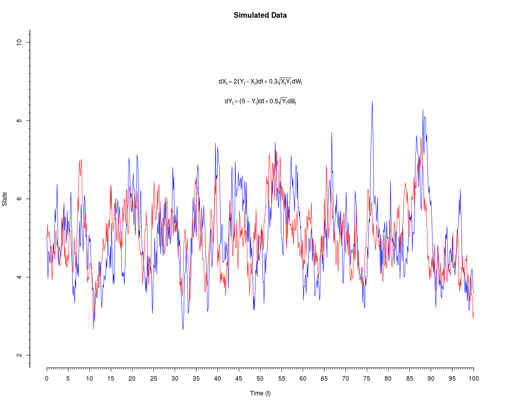
  # Have a look at the time series:
  plot(Xt~time,type='l',col='blue',ylim=c(2,10),main='Simulated Data',xlab='Time (t)',ylab='State',
       axes=FALSE)
  lines(Yt~time,col='red')
  expr1=expression(dX[t]==2(Y[t]-X[t])*dt+0.3*sqrt(X[t]*Y[t])*dW[t])
  expr2=expression(dY[t]==(5-Y[t])*dt+0.5*sqrt(Y[t])*dB[t])
  text(50,9,expr1)
  text(50,8.5,expr2)
  axis(1,seq(0,100,5))
  axis(1,seq(0,100,5/10),tcl=-0.2,labels=NA)
  axis(2,seq(0,20,2))
  axis(2,seq(0,20,2/10),tcl=-0.2,labels=NA)

 #------------------------------------------------------------------------------
 # Define the coefficients of a proposed model
 #------------------------------------------------------------------------------
  GQD.remove()
  a00 <- function(t){theta[1]*theta[2]}
  a10 <- function(t){-theta[1]}
  c00 <- function(t){theta[3]*theta[3]}

  b00 <- function(t){theta[4]}
  b01 <- function(t){-theta[5]}
  f00 <- function(t){theta[6]*theta[6]}

  theta.start <- c(3,3,3,3,3,3)
  prop.sds    <- c(0.15,0.16,0.04,0.99,0.19,0.04)
  updates     <- 50000
  X           <- cbind(Xt,Yt)
  
  # Define prior distributions:
  priors=function(theta){dunif(theta[1],0,100)*dunif(theta[4],0,100)}
  
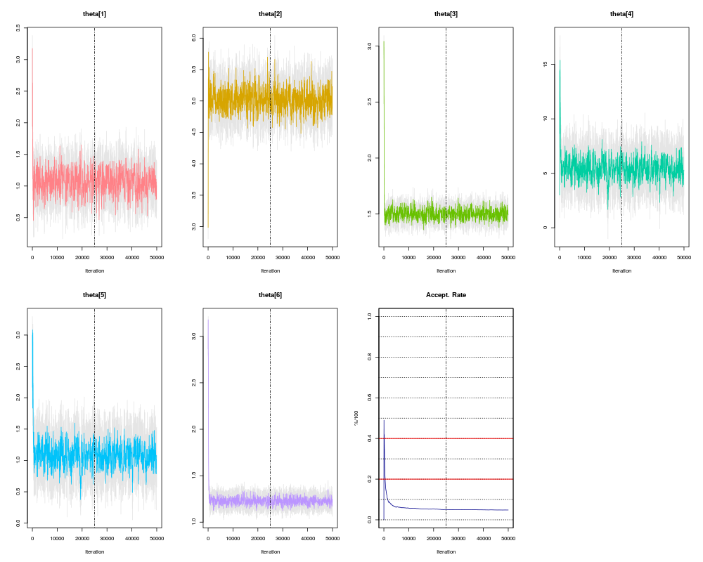
  # Run the MCMC procedure
  m1=BiGQD.mcmc(X,time,10,theta.start,prop.sds,updates)

 #------------------------------------------------------------------------------
 # Remove old coefficients and define the coefficients of a new model
 #------------------------------------------------------------------------------
  GQD.remove()
  a10 <- function(t){-theta[1]}
  a01 <- function(t){theta[1]*theta[2]}
  c11 <- function(t){theta[3]*theta[3]}

  b00 <- function(t){theta[4]*theta[5]}
  b01 <- function(t){-theta[4]}
  f01 <- function(t){theta[6]*theta[6]}

  theta.start <- c(3,3,3,3,3,3)
  prop.sds    <- c(0.16,0.02,0.01,0.18,0.12,0.01)

  # Define prior distributions:
  priors=function(theta){dunif(theta[1],0,100)*dunif(theta[4],0,100)}

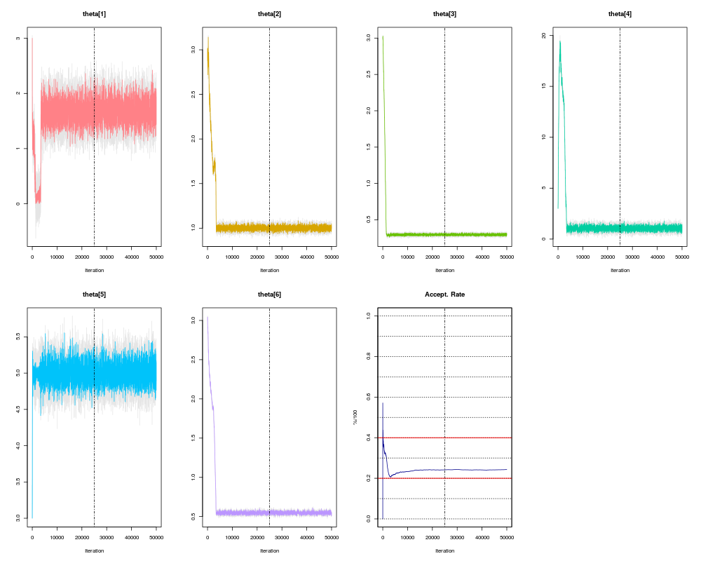
  # Run the MCMC procedure
  m2=BiGQD.mcmc(X,time,10,theta.start,prop.sds,updates)

 # Compare estimates:
  GQD.estimates(m1)
  GQD.estimates(m2)

 #------------------------------------------------------------------------------
 # Compare the two models
 #------------------------------------------------------------------------------

  GQD.dic(list(m1,m2))


#===============================================================================

Results


R version 3.3.1 (2016-06-21) -- "Bug in Your Hair"
Copyright (C) 2016 The R Foundation for Statistical Computing
Platform: x86_64-pc-linux-gnu (64-bit)

R is free software and comes with ABSOLUTELY NO WARRANTY.
You are welcome to redistribute it under certain conditions.
Type 'license()' or 'licence()' for distribution details.

R is a collaborative project with many contributors.
Type 'contributors()' for more information and
'citation()' on how to cite R or R packages in publications.

Type 'demo()' for some demos, 'help()' for on-line help, or
'help.start()' for an HTML browser interface to help.
Type 'q()' to quit R.

> library(DiffusionRgqd)
> png(filename="/home/ddbj/snapshot/RGM3/R_CC/result/DiffusionRgqd/BiGQD.mcmc.Rd_%03d_medium.png", width=480, height=480)
> ### Name: BiGQD.mcmc
> ### Title: MCMC Inference on Bivariate Generalized Quadratic Diffusions (2D
> ###   GQDs).
> ### Aliases: BiGQD.mcmc
> ### Keywords: syntax C++ MCMC
> 
> ### ** Examples
> 
> ## No test: 
> #===============================================================================
> # This example simulates a bivariate time homogeneous diffusion and shows how
> # to conduct inference using BiGQD.mcmc(). We fit two competing models and then
> # use the output to select a winner.
> #-------------------------------------------------------------------------------
> 
>   data(SDEsim2)
>   data(SDEsim2)
>   attach(SDEsim2)
>   # Have a look at the time series:
>   plot(Xt~time,type='l',col='blue',ylim=c(2,10),main='Simulated Data',xlab='Time (t)',ylab='State',
+        axes=FALSE)
>   lines(Yt~time,col='red')
>   expr1=expression(dX[t]==2(Y[t]-X[t])*dt+0.3*sqrt(X[t]*Y[t])*dW[t])
>   expr2=expression(dY[t]==(5-Y[t])*dt+0.5*sqrt(Y[t])*dB[t])
>   text(50,9,expr1)
>   text(50,8.5,expr2)
>   axis(1,seq(0,100,5))
>   axis(1,seq(0,100,5/10),tcl=-0.2,labels=NA)
>   axis(2,seq(0,20,2))
>   axis(2,seq(0,20,2/10),tcl=-0.2,labels=NA)
> 
>  #------------------------------------------------------------------------------
>  # Define the coefficients of a proposed model
>  #------------------------------------------------------------------------------
>   GQD.remove()
[1] "Removed :  NA "
>   a00 <- function(t){theta[1]*theta[2]}
>   a10 <- function(t){-theta[1]}
>   c00 <- function(t){theta[3]*theta[3]}
> 
>   b00 <- function(t){theta[4]}
>   b01 <- function(t){-theta[5]}
>   f00 <- function(t){theta[6]*theta[6]}
> 
>   theta.start <- c(3,3,3,3,3,3)
>   prop.sds    <- c(0.15,0.16,0.04,0.99,0.19,0.04)
>   updates     <- 50000
>   X           <- cbind(Xt,Yt)
>   
>   # Define prior distributions:
>   priors=function(theta){dunif(theta[1],0,100)*dunif(theta[4],0,100)}
>   
>   # Run the MCMC procedure
>   m1=BiGQD.mcmc(X,time,10,theta.start,prop.sds,updates)
Compiling C++ code. Please wait.                                                                                                           
 ================================================================
                   GENERALIZED LINEAR DIFFUSON                   
 ================================================================
 _____________________ Drift Coefficients _______________________
 a00 : theta[1]*theta[2]                                         
 a10 : -theta[1]                                                 
 ...   ...   ...   ...   ...   ...   ...   ...   ...   ...   ... 
 b00 : theta[4]                                                  
 b01 : -theta[5]                                                 
 ___________________ Diffusion Coefficients _____________________
 c00 : theta[3]*theta[3]                                         
 ...   ...   ...   ...   ...   ...   ...   ...   ...   ...   ... 
 ...   ...   ...   ...   ...   ...   ...   ...   ...   ...   ... 
 ...   ...   ...   ...   ...   ...   ...   ...   ...   ...   ... 
 f00 : theta[6]*theta[6]                                         
 _____________________ Prior Distributions ______________________
                                                                 
 d(theta):dunif(theta[1],0,100)*dunif(theta[4],0,100)            
=================================================================
                                                                 
 _______________________ Model/Chain Info _______________________
 Chain Updates       : 50000                                     
 Burned Updates      : 25000                                     
 Time Homogeneous    : Yes                                       
 Data Resolution     : Homogeneous: dt=0.125                     
 # Removed Transits. : None                                      
 Density approx.     : 2nd Ord. Truncation, Bivariate Normal     
 Elapsed time        : 00:01:05                                  
 ...   ...   ...   ...   ...   ...   ...   ...   ...   ...   ... 
 dim(theta)          : 6                                         
 DIC                 : 1833.787                                  
 pd (eff. dim(theta)): 5.876                                     
 ----------------------------------------------------------------
> 
>  #------------------------------------------------------------------------------
>  # Remove old coefficients and define the coefficients of a new model
>  #------------------------------------------------------------------------------
>   GQD.remove()
[1] "Removed :  a00 a10 b00 b01 c00 f00 priors"
>   a10 <- function(t){-theta[1]}
>   a01 <- function(t){theta[1]*theta[2]}
>   c11 <- function(t){theta[3]*theta[3]}
> 
>   b00 <- function(t){theta[4]*theta[5]}
>   b01 <- function(t){-theta[4]}
>   f01 <- function(t){theta[6]*theta[6]}
> 
>   theta.start <- c(3,3,3,3,3,3)
>   prop.sds    <- c(0.16,0.02,0.01,0.18,0.12,0.01)
> 
>   # Define prior distributions:
>   priors=function(theta){dunif(theta[1],0,100)*dunif(theta[4],0,100)}
> 
>   # Run the MCMC procedure
>   m2=BiGQD.mcmc(X,time,10,theta.start,prop.sds,updates)
Compiling C++ code. Please wait.                                                                                                           
 ================================================================
                   GENERALIZED QUADRATIC DIFFUSON                
 ================================================================
 _____________________ Drift Coefficients _______________________
 a10 : -theta[1]                                                 
 a01 : theta[1]*theta[2]                                         
 ...   ...   ...   ...   ...   ...   ...   ...   ...   ...   ... 
 b00 : theta[4]*theta[5]                                         
 b01 : -theta[4]                                                 
 ___________________ Diffusion Coefficients _____________________
 c11 : theta[3]*theta[3]                                         
 ...   ...   ...   ...   ...   ...   ...   ...   ...   ...   ... 
 ...   ...   ...   ...   ...   ...   ...   ...   ...   ...   ... 
 ...   ...   ...   ...   ...   ...   ...   ...   ...   ...   ... 
 f01 : theta[6]*theta[6]                                         
 _____________________ Prior Distributions ______________________
                                                                 
 d(theta):dunif(theta[1],0,100)*dunif(theta[4],0,100)            
=================================================================
                                                                 
 _______________________ Model/Chain Info _______________________
 Chain Updates       : 50000                                     
 Burned Updates      : 25000                                     
 Time Homogeneous    : Yes                                       
 Data Resolution     : Homogeneous: dt=0.125                     
 # Removed Transits. : None                                      
 Density approx.     : 4th Ord. Truncation, Bivariate-Saddlepoint
 Elapsed time        : 00:03:13                                  
 ...   ...   ...   ...   ...   ...   ...   ...   ...   ...   ... 
 dim(theta)          : 6                                         
 DIC                 : 1729.019                                  
 pd (eff. dim(theta)): 6.041                                     
 ----------------------------------------------------------------
> 
>  # Compare estimates:
>   GQD.estimates(m1)
         Estimate Lower_CI Upper_CI
theta[1]    1.042    0.800    1.295
theta[2]    5.013    4.766    5.277
theta[3]    1.493    1.434    1.554
theta[4]    5.262    4.078    6.585
theta[5]    1.054    0.812    1.312
theta[6]    1.226    1.175    1.282
>   GQD.estimates(m2)
         Estimate Lower_CI Upper_CI
theta[1]    1.659    1.377    1.953
theta[2]    1.002    0.970    1.032
theta[3]    0.296    0.283    0.308
theta[4]    1.044    0.766    1.322
theta[5]    4.992    4.788    5.234
theta[6]    0.547    0.524    0.575
> 
>  #------------------------------------------------------------------------------
>  # Compare the two models
>  #------------------------------------------------------------------------------
> 
>   GQD.dic(list(m1,m2))
        Elapsed_Time Time_Homogeneous        p           DIC       pD   N
Model 1     00:01:05              Yes    6.000      1833.790    5.880 801
Model 2     00:03:13              Yes    6.000  [=] 1729.020    6.040 801
> 
> 
> #===============================================================================
>  
> ## End(No test)
>  
> 
> 
> 
> 
> dev.off()
null device 
          1 
>