R Graphical Manual

Browse All

Last data update: 2014.03.03

R: Calculate Maximum Likelihood Estimates for a 2D GQD Model.

BiGQD.mle

R Documentation

Calculate Maximum Likelihood Estimates for a 2D GQD Model.

Description

BiGQD.mle() uses parametrised coefficients (provided by the user as R-functions) to construct a C++ program in real time that allows the user to perform maximum likelihood inference on the resulting diffusion model. BiGQD.density generates approximate transitional densities for a class of bivariate diffusion processes with SDE:

where

and

Usage

BiGQD.mle(X, time, mesh=10, theta, control=NULL, method='Nelder-Mead', RK.order=4,
          exclude=NULL, Tag=NA, Dtype='Saddlepoint', rtf= runif(2,-1,1), wrt=FALSE,
          print.output=TRUE)

Arguments

`X`	A matrix containing rows of data points to be modelled. Though observations are allowed to be non-equidistant, observations in both dimensions are assumed to occur at the same time epochs.
`time`	A vector containing the time epochs at which observations were made.
`mesh`	The number of mesh points in the time discretisation.
`theta`	The parameter vector starting values.
`control`	List of control variables to be used by `optim`.
`method`	Method to be used by `optim`.
`exclude`	Vector indicating which transitions to exclude from the analysis. Default = `NULL`.
`RK.order`	The order of the Runge-Kutta solver used to approximate the trajectories of cumulants. Must be 4 (default) or 10.
`Tag`	`Tag` can be used to name (tag) an MCMC run e.g. `Tag='Run_1'`
`Dtype`	The density approximant to use. Valid types are `"Saddlepoint"` (default), `"Edgeworth"` or `"Normal"`.
`rtf`	Starting vector for internal use.
`wrt`	If `TRUE` a .cpp file will be written to the current directory. For bug report diagnostics.
`print.output`	If `TRUE` information about the model and algorithm is printed to the console.

Value

`opt`	The output from optim.
`model.info`	A list of variables pertaining to inference calculations.
`model.info$elapsed.time`	The runtime, in h/m/s format,of the MCMC procedure (excluding compile time).
`model.info$time.homogeneous`	‘No’ if the model has time-homogeneous coefficients and ‘Yes’ otherwise.
`model.info$p`	The dimension of `theta`.

Syntactical jargon

Synt. [1]: The coefficients of the 2D GQD may be parameterized using the reserved variable theta. For example:

a00 <- function(t){theta[1]*(theta[2]+sin(2*pi*(t-theta[3])))}.

Synt. [2]: Due to syntactical differences between R and C++ special functions have to be used when terms that depend on t. When the function cannot be separated in to terms that contain a single t, the prod(a,b) function must be used. For example:

a00 <- function(t){0.1*(10+0.2*sin(2*pi*t)+0.3*prod(sqrt(t),1+cos(3*pi*t)))}.

Here sqrt(t)*cos(3*pi*t) constitutes the product of two terms that cannot be written i.t.o. a single t. To circumvent this isue, one may use the prod(a,b) function.

Synt. [3]: Similarly, the ^ - operator is not overloaded in C++. Instead the pow(x,p) function may be used to calculate x^p. For example sin(2*pi*t)^3 in:

a00 <- function(t){0.1*(10+0.2*pow(sin(2*pi*t),3))}.

Warning

Warning [1]: The parameter mesh is used to discretize the transition horizons between successive observations. It is thus important to ensure that mesh is not too small when large time differences are present in time. Check output for max(dt) and divide by mesh.

Warning [2]: Note that minus the likelihood is minimized, as such the optim output (hessian) needs to be adjusted accordingly if used for calculating confidence intervals. Furthermore, GQD.mle may be temperamental under certain conditions

Author(s)

Etienne A.D. Pienaar: etiennead@gmail.com

References

Updates available on GitHub at https://github.com/eta21.

Daniels, H.E. 1954 Saddlepoint approximations in statistics. Ann. Math. Stat., 25:631–650.

Eddelbuettel, D. and Romain, F. 2011 Rcpp: Seamless R and C++ integration. Journal of Statistical Software, 40(8):1–18,. URL http://www.jstatsoft.org/v40/i08/.

Eddelbuettel, D. 2013 Seamless R and C++ Integration with Rcpp. New York: Springer. ISBN 978-1-4614-6867-7.

Eddelbuettel, D. and Sanderson, C. 2014 Rcpparmadillo: Accelerating R with high-performance C++ linear algebra. Computational Statistics and Data Analysis, 71:1054–1063. URL http://dx.doi.org/10.1016/j.csda.2013.02.005.

Feagin, T. 2007 A tenth-order Runge-Kutta method with error estimate. In Proceedings of the IAENG Conf. on Scientifc Computing.

Varughese, M.M. 2013 Parameter estimation for multivariate diffusion systems. Comput. Stat. Data An., 57:417–428.

Examples


#===============================================================================
# This example simulates a bivariate time homogeneous diffusion and shows how
# to conduct inference using BiGQD.mle(). We fit two competing models and then
# use the output to select a winner.
#-------------------------------------------------------------------------------

  data(SDEsim2)
  data(SDEsim2)
  attach(SDEsim2)
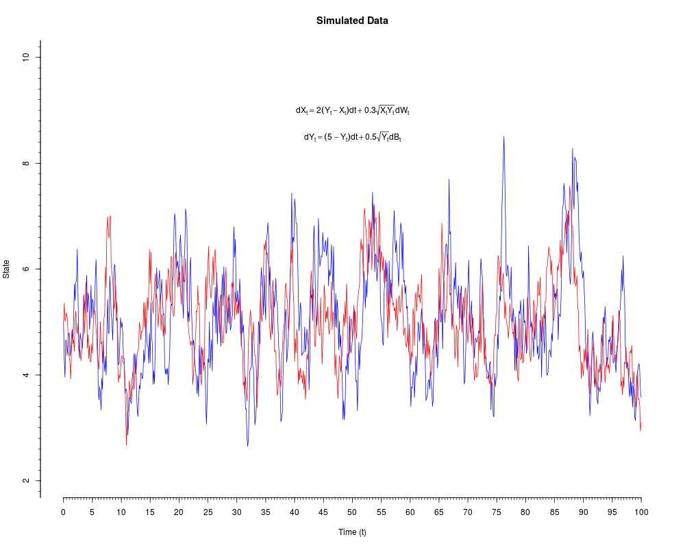
  # Have a look at the time series:
  plot(Xt~time,type='l',col='blue',ylim=c(2,10),main='Simulated Data',xlab='Time (t)',ylab='State',
       axes=FALSE)
  lines(Yt~time,col='red')
  expr1=expression(dX[t]==2(Y[t]-X[t])*dt+0.3*sqrt(X[t]*Y[t])*dW[t])
  expr2=expression(dY[t]==(5-Y[t])*dt+0.5*sqrt(Y[t])*dB[t])
  text(50,9,expr1)
  text(50,8.5,expr2)
  axis(1,seq(0,100,5))
  axis(1,seq(0,100,5/10),tcl=-0.2,labels=NA)
  axis(2,seq(0,20,2))
  axis(2,seq(0,20,2/10),tcl=-0.2,labels=NA)

 #------------------------------------------------------------------------------
 # Define the coefficients of a proposed model
 #------------------------------------------------------------------------------
  GQD.remove()
  a00 <- function(t){theta[1]*theta[2]}
  a10 <- function(t){-theta[1]}
  c00 <- function(t){theta[3]*theta[3]}

  b00 <- function(t){theta[4]}
  b01 <- function(t){-theta[5]}
  f00 <- function(t){theta[6]*theta[6]}

  theta.start <- c(3,3,3,3,3,3)
  X           <- cbind(Xt,Yt)

  # Calculate MLEs
  m1=BiGQD.mle(X,time,10,theta.start)

 #------------------------------------------------------------------------------
 # Remove old coefficients and define the coefficients of a new model
 #------------------------------------------------------------------------------
  GQD.remove()
  a10 <- function(t){-theta[1]}
  a01 <- function(t){theta[1]*theta[2]}
  c11 <- function(t){theta[3]*theta[3]}

  b00 <- function(t){theta[4]*theta[5]}
  b01 <- function(t){-theta[4]}
  f01 <- function(t){theta[6]*theta[6]}

  theta.start <- c(3,3,3,3,3,3)

  # Calculate MLEs
  m2=BiGQD.mle(X,time,10,theta.start)

 # Compare estimates:
  GQD.estimates(m1)
  GQD.estimates(m2)

 #------------------------------------------------------------------------------
 # Compare the two models
 #------------------------------------------------------------------------------

  GQD.aic(list(m1,m2))


#===============================================================================

Results


R version 3.3.1 (2016-06-21) -- "Bug in Your Hair"
Copyright (C) 2016 The R Foundation for Statistical Computing
Platform: x86_64-pc-linux-gnu (64-bit)

R is free software and comes with ABSOLUTELY NO WARRANTY.
You are welcome to redistribute it under certain conditions.
Type 'license()' or 'licence()' for distribution details.

R is a collaborative project with many contributors.
Type 'contributors()' for more information and
'citation()' on how to cite R or R packages in publications.

Type 'demo()' for some demos, 'help()' for on-line help, or
'help.start()' for an HTML browser interface to help.
Type 'q()' to quit R.

> library(DiffusionRgqd)
> png(filename="/home/ddbj/snapshot/RGM3/R_CC/result/DiffusionRgqd/BiGQD.mle.Rd_%03d_medium.png", width=480, height=480)
> ### Name: BiGQD.mle
> ### Title: Calculate Maximum Likelihood Estimates for a 2D GQD Model.
> ### Aliases: BiGQD.mle
> ### Keywords: syntax C++ maximum likelihood
> 
> ### ** Examples
> 
> ## No test: 
> #===============================================================================
> # This example simulates a bivariate time homogeneous diffusion and shows how
> # to conduct inference using BiGQD.mle(). We fit two competing models and then
> # use the output to select a winner.
> #-------------------------------------------------------------------------------
> 
>   data(SDEsim2)
>   data(SDEsim2)
>   attach(SDEsim2)
>   # Have a look at the time series:
>   plot(Xt~time,type='l',col='blue',ylim=c(2,10),main='Simulated Data',xlab='Time (t)',ylab='State',
+        axes=FALSE)
>   lines(Yt~time,col='red')
>   expr1=expression(dX[t]==2(Y[t]-X[t])*dt+0.3*sqrt(X[t]*Y[t])*dW[t])
>   expr2=expression(dY[t]==(5-Y[t])*dt+0.5*sqrt(Y[t])*dB[t])
>   text(50,9,expr1)
>   text(50,8.5,expr2)
>   axis(1,seq(0,100,5))
>   axis(1,seq(0,100,5/10),tcl=-0.2,labels=NA)
>   axis(2,seq(0,20,2))
>   axis(2,seq(0,20,2/10),tcl=-0.2,labels=NA)
> 
>  #------------------------------------------------------------------------------
>  # Define the coefficients of a proposed model
>  #------------------------------------------------------------------------------
>   GQD.remove()
[1] "Removed :  NA "
>   a00 <- function(t){theta[1]*theta[2]}
>   a10 <- function(t){-theta[1]}
>   c00 <- function(t){theta[3]*theta[3]}
> 
>   b00 <- function(t){theta[4]}
>   b01 <- function(t){-theta[5]}
>   f00 <- function(t){theta[6]*theta[6]}
> 
>   theta.start <- c(3,3,3,3,3,3)
>   X           <- cbind(Xt,Yt)
> 
>   # Calculate MLEs
>   m1=BiGQD.mle(X,time,10,theta.start)
Compiling C++ code. Please wait.                                                                                                           
 ================================================================
                   GENERALIZED LINEAR DIFFUSON                   
 ================================================================
 _____________________ Drift Coefficients _______________________
 a00 : theta[1]*theta[2]                                         
 a10 : -theta[1]                                                 
 ...   ...   ...   ...   ...   ...   ...   ...   ...   ...   ... 
 b00 : theta[4]                                                  
 b01 : -theta[5]                                                 
 ___________________ Diffusion Coefficients _____________________
 c00 : theta[3]*theta[3]                                         
 ...   ...   ...   ...   ...   ...   ...   ...   ...   ...   ... 
 ...   ...   ...   ...   ...   ...   ...   ...   ...   ...   ... 
 ...   ...   ...   ...   ...   ...   ...   ...   ...   ...   ... 
 f00 : theta[6]*theta[6]                                         
                                                                 
 __________________________ Model Info __________________________
 Time Homogeneous    : Yes                                       
 Data Resolution     : Homogeneous: dt=0.125                     
 # Removed Transits. : None                                      
 Density approx.     : 2nd Ord. Truncation, Bivariate Normal     
 Elapsed time        : 00:00:01                                  
 ...   ...   ...   ...   ...   ...   ...   ...   ...   ...   ... 
 dim(theta)          : 6                                         
 ----------------------------------------------------------------
> 
>  #------------------------------------------------------------------------------
>  # Remove old coefficients and define the coefficients of a new model
>  #------------------------------------------------------------------------------
>   GQD.remove()
[1] "Removed :  a00 a10 b00 b01 c00 f00"
>   a10 <- function(t){-theta[1]}
>   a01 <- function(t){theta[1]*theta[2]}
>   c11 <- function(t){theta[3]*theta[3]}
> 
>   b00 <- function(t){theta[4]*theta[5]}
>   b01 <- function(t){-theta[4]}
>   f01 <- function(t){theta[6]*theta[6]}
> 
>   theta.start <- c(3,3,3,3,3,3)
> 
>   # Calculate MLEs
>   m2=BiGQD.mle(X,time,10,theta.start)
Compiling C++ code. Please wait.                                                                                                           
 ================================================================
                   GENERALIZED QUADRATIC DIFFUSON                
 ================================================================
 _____________________ Drift Coefficients _______________________
 a10 : -theta[1]                                                 
 a01 : theta[1]*theta[2]                                         
 ...   ...   ...   ...   ...   ...   ...   ...   ...   ...   ... 
 b00 : theta[4]*theta[5]                                         
 b01 : -theta[4]                                                 
 ___________________ Diffusion Coefficients _____________________
 c11 : theta[3]*theta[3]                                         
 ...   ...   ...   ...   ...   ...   ...   ...   ...   ...   ... 
 ...   ...   ...   ...   ...   ...   ...   ...   ...   ...   ... 
 ...   ...   ...   ...   ...   ...   ...   ...   ...   ...   ... 
 f01 : theta[6]*theta[6]                                         
                                                                 
 __________________________ Model Info __________________________
 Time Homogeneous    : Yes                                       
 Data Resolution     : Homogeneous: dt=0.125                     
 # Removed Transits. : None                                      
 Density approx.     : 4th Ord. Truncation, Bivariate-Saddlepoint
 Elapsed time        : 00:00:07                                  
 ...   ...   ...   ...   ...   ...   ...   ...   ...   ...   ... 
 dim(theta)          : 6                                         
 ----------------------------------------------------------------
> 
>  # Compare estimates:
>   GQD.estimates(m1)
         Estimate Lower_95 Upper_95
theta[1]    1.073    0.749    1.397
theta[2]    5.023    4.735    5.311
theta[3]    1.495    1.418    1.573
theta[4]    5.377    3.714    7.040
theta[5]    1.075    0.748    1.403
theta[6]    1.224    1.160    1.287
>   GQD.estimates(m2)
         Estimate Lower_95 Upper_95
theta[1]    5.639      NaN      NaN
theta[2]    0.994    0.978    1.010
theta[3]    0.421      NaN      NaN
theta[4]    3.077    2.361    3.792
theta[5]    5.079    4.968    5.189
theta[6]    0.660    0.601    0.719
Warning message:
In sqrt(diag(solve(-x$opt$hessian))) : NaNs produced
> 
>  #------------------------------------------------------------------------------
>  # Compare the two models
>  #------------------------------------------------------------------------------
> 
>   GQD.aic(list(m1,m2))
        Convergence p min.likelihood           AIC           BIC   N
Model 1           0 6       910.9934  [=] 1833.987  [=] 1862.102 801
Model 2           0 6      1047.7193     2107.4385     2135.5537 801
> 
> 
> #===============================================================================
> ## End(No test)
> 
> 
> 
> 
> 
> dev.off()
null device 
          1 
>