Summarize MLE Selection Output for a List of GQD.mle or BiGQD.mle objects.

Description

GQD.aic() summarizes the MCMC output from a list of GQD.mle() objects. This may be used to neatly summarize the MCMC output of various models fitted to a given dataset.

Usage

GQD.aic(model.list, type = "col")

Arguments

Details

GQD.aic() summarizes the output from various models fitted via GQD.mle(). By ranking them according to DIC. [=] indicates which model has the minimal DIC.

Value

Author(s)

Etienne A.D. Pienaar: etiannead@gmail.com

References

Updates available on GitHub at https://github.com/eta21.

See Also

GQD.mle

Examples

#===============================================================================
# Simulate a time inhomogeneous diffusion.
#-------------------------------------------------------------------------------

  data(SDEsim1)
  attach(SDEsim1)
  par(mfrow=c(1,1))
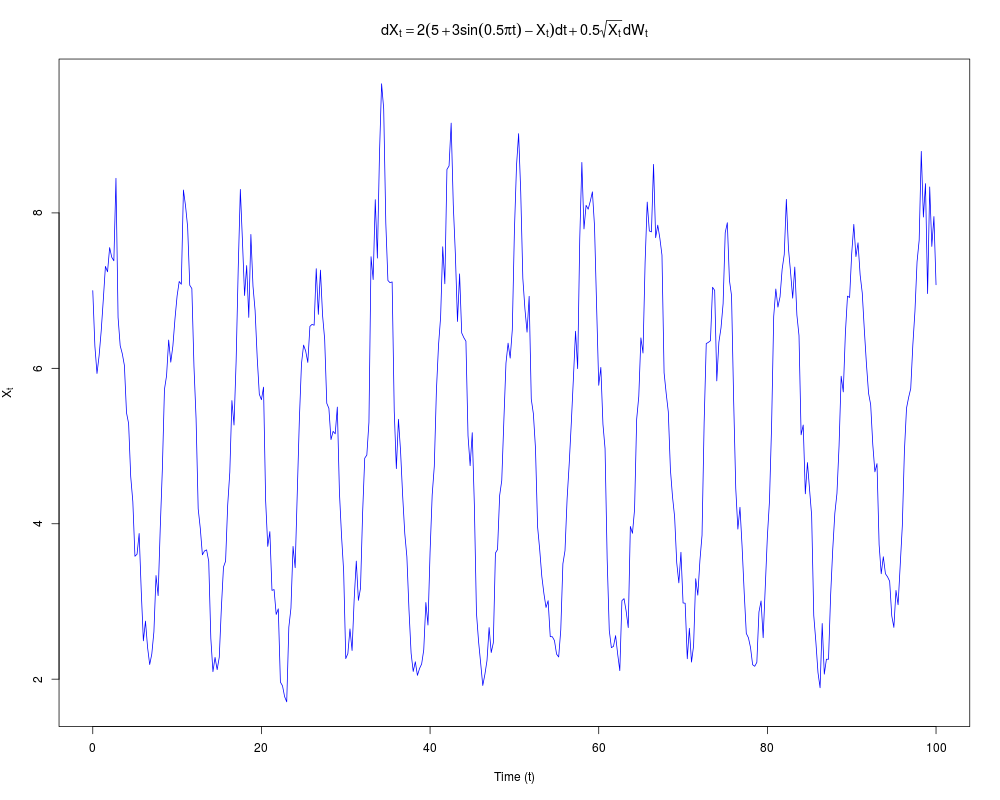
  expr1=expression(dX[t]==2*(5+3*sin(0.5*pi*t)-X[t])*dt+0.5*sqrt(X[t])*dW[t])
  plot(Xt~time,type='l',col='blue',xlab='Time (t)',ylab=expression(X[t]),main=expr1)

 #------------------------------------------------------------------------------
 # Define coefficients of the process.
 #------------------------------------------------------------------------------

  GQD.remove()
  G0 <- function(t){theta[1]*(theta[2]+theta[3]*sin(0.25*pi*t))}
  G1 <- function(t){-theta[1]}
  Q0 <- function(t){theta[4]*theta[4]}

  theta.start  <- c(1,1,1,1)                      # Starting values for the chain
  mesh.points  <- 10                              # Number of mesh points

  m1 <- GQD.mle(Xt,time,mesh=mesh.points,theta=theta.start)

  GQD.remove()

  G1 <- function(t){theta[1]*(theta[2]+theta[3]*sin(0.25*pi*t))}
  G2 <- function(t){-theta[1]}
  Q2 <- function(t){theta[4]*theta[4]}

  theta.start  <- c(1,1,1,1)                      # Starting values for the chain
  mesh.points  <- 10                              # Number of mesh points

  m2 <- GQD.mle(Xt,time,mesh=mesh.points,theta=theta.start)

  # Check estimates:
  GQD.estimates(m1)
  GQD.estimates(m2)

  # Compare models:
  GQD.aic(list(m1,m2))

#===============================================================================

Results

R version 3.3.1 (2016-06-21) -- "Bug in Your Hair"
Copyright (C) 2016 The R Foundation for Statistical Computing
Platform: x86_64-pc-linux-gnu (64-bit)

R is free software and comes with ABSOLUTELY NO WARRANTY.
You are welcome to redistribute it under certain conditions.
Type 'license()' or 'licence()' for distribution details.

R is a collaborative project with many contributors.
Type 'contributors()' for more information and
'citation()' on how to cite R or R packages in publications.

Type 'demo()' for some demos, 'help()' for on-line help, or
'help.start()' for an HTML browser interface to help.
Type 'q()' to quit R.

> library(DiffusionRgqd)
> png(filename="/home/ddbj/snapshot/RGM3/R_CC/result/DiffusionRgqd/GQD.aic.Rd_%03d_medium.png", width=480, height=480)
> ### Name: GQD.aic
> ### Title: Summarize MLE Selection Output for a List of GQD.mle or
> ###   BiGQD.mle objects.
> ### Aliases: GQD.aic
> ### Keywords: Akaike information criterion (AIC) Bayesian information
> ###   criterion (BIC)
> 
> ### ** Examples
> 
> ## No test: 
> #===============================================================================
> # Simulate a time inhomogeneous diffusion.
> #-------------------------------------------------------------------------------
> 
>   data(SDEsim1)
>   attach(SDEsim1)
>   par(mfrow=c(1,1))
>   expr1=expression(dX[t]==2*(5+3*sin(0.5*pi*t)-X[t])*dt+0.5*sqrt(X[t])*dW[t])
>   plot(Xt~time,type='l',col='blue',xlab='Time (t)',ylab=expression(X[t]),main=expr1)
> 
>  #------------------------------------------------------------------------------
>  # Define coefficients of the process.
>  #------------------------------------------------------------------------------
> 
>   GQD.remove()
[1] "Removed :  NA "
>   G0 <- function(t){theta[1]*(theta[2]+theta[3]*sin(0.25*pi*t))}
>   G1 <- function(t){-theta[1]}
>   Q0 <- function(t){theta[4]*theta[4]}
> 
>   theta.start  <- c(1,1,1,1)                      # Starting values for the chain
>   mesh.points  <- 10                              # Number of mesh points
> 
>   m1 <- GQD.mle(Xt,time,mesh=mesh.points,theta=theta.start)
Compiling C++ code. Please wait.                                                                                                           
 ================================================================
                  Generalized Ornstein-Uhlenbeck                 
 ================================================================
 _____________________ Drift Coefficients _______________________
 G0 : theta[1]*(theta[2]+theta[3]*sin(0.25*pi*t))                
 G1 : -theta[1]                                                  
 G2                                                              
 ___________________ Diffusion Coefficients _____________________
 Q0 : theta[4]*theta[4]                                          
 Q1                                                              
 Q2                                                              
                                                                 
 _______________________ Model/Chain Info _______________________
 Time Homogeneous    : No                                        
 Data Resolution     : Homogeneous: dt=0.25                      
 # Removed Transits. : None                                      
 Density approx.     : 2nd Ord. Truncation + Std Normal Dist.    
 Elapsed time        : 00:00:00                                  
 ...   ...   ...   ...   ...   ...   ...   ...   ...   ...   ... 
 dim(theta)          : 4                                         
 ----------------------------------------------------------------
> 
>   GQD.remove()
[1] "Removed :  G0 G1 Q0"
> 
>   G1 <- function(t){theta[1]*(theta[2]+theta[3]*sin(0.25*pi*t))}
>   G2 <- function(t){-theta[1]}
>   Q2 <- function(t){theta[4]*theta[4]}
> 
>   theta.start  <- c(1,1,1,1)                      # Starting values for the chain
>   mesh.points  <- 10                              # Number of mesh points
> 
>   m2 <- GQD.mle(Xt,time,mesh=mesh.points,theta=theta.start)
Compiling C++ code. Please wait.                                                                                                           
 ================================================================
                  Generalized Quadratic Diffusion (GQD)          
 ================================================================
 _____________________ Drift Coefficients _______________________
 G0                                                              
 G1 : theta[1]*(theta[2]+theta[3]*sin(0.25*pi*t))                
 G2 : -theta[1]                                                  
 ___________________ Diffusion Coefficients _____________________
 Q0                                                              
 Q1                                                              
 Q2 : theta[4]*theta[4]                                          
                                                                       
 _______________________ Model/Chain Info _______________________      
 Time Homogeneous    : No                                              
 Data Resolution     : Homogeneous: dt=0.25                            
 # Removed Transits. : None                                            
 Density approx.     : 4 Ord. Truncation +4th Ord. Saddlepoint Appr.   
 Elapsed time        : 00:00:01                                        
 ...   ...   ...   ...   ...   ...   ...   ...   ...   ...   ...       
 dim(theta)          : 4                                               
 ----------------------------------------------------------------      
> 
>   # Check estimates:
>   GQD.estimates(m1)
         Estimate Lower_95 Upper_95
theta[1]    2.087    1.804    2.369
theta[2]    5.016    4.908    5.124
theta[3]    2.899    2.738    3.059
theta[4]    1.138    1.052    1.223
>   GQD.estimates(m2)
         Estimate Lower_95 Upper_95
theta[1]    0.034      NaN      NaN
theta[2]    1.980      NaN      NaN
theta[3]    7.669    5.961    9.378
theta[4]    0.264    0.246    0.283
Warning message:
In sqrt(diag(solve(-x$opt$hessian))) : NaNs produced
> 
>   # Compare models:
>   GQD.aic(list(m1,m2))
        Convergence p min.likelihood           AIC          BIC   N
Model 1           0 4       246.5406  [=] 501.0812  [=] 517.057 401
Model 2           0 4       375.9415      759.8829     775.8588 401
> 
> #===============================================================================
> ## End(No test)
> 
> 
> 
> 
> 
> dev.off()
null device 
          1 
>