Summarize MCMC Selection Output for a List of GQD.mcmc or BiGQD.mcmc objects.

Description

GQD.dic() summarizes the MCMC output from a list of GQD.mcmc() objects. This may be used to neatly summarize the MCMC output of various models fitted to a given dataset.

Usage

GQD.dic(model.list, type = "col")

Arguments

Details

GQD.dic() summarizes the output from various models fitted via GQD.mcmc(). By ranking them according to DIC. [=] indicates which model has the minimal DIC.

Value

Author(s)

Etienne A.D. Pienaar: etiannead@gmail.com

References

Updates available on GitHub at https://github.com/eta21.

See Also

GQD.mcmc

Examples

#===============================================================================
# Simulate a time inhomogeneous diffusion.
#-------------------------------------------------------------------------------

 data(SDEsim1)
 attach(SDEsim1)
 par(mfrow=c(1,1))
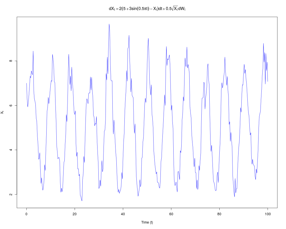
 expr1=expression(dX[t]==2*(5+3*sin(0.5*pi*t)-X[t])*dt+0.5*sqrt(X[t])*dW[t])
 plot(Xt~time,type='l',col='blue',xlab='Time (t)',ylab=expression(X[t]),main=expr1)


 #------------------------------------------------------------------------------
 # Define coefficients of model 1
 #------------------------------------------------------------------------------

  # Remove any existing coeffients. If none are pressent NAs will be returned, but
  # this is a safeguard against overlapping.
    GQD.remove()

  # Define time dependant coefficients. Note that all functions have a single argument.
  # This argument has to be `t' in order for the dependancy to be recognized.
  # theta does not have to be defined as an argument.

  G0 <- function(t){theta[1]*(theta[2]+theta[3]*sin(0.25*pi*t))}
  G1 <- function(t){-theta[1]}
  Q0 <- function(t){theta[4]*theta[4]}

  theta.start   <-  c(1,1,1,1)                     # Starting values for the chain
  proposal.sds  <-  c(0.8,0.1,0.1,0.1)             # Std devs for proposal distributions
  mesh.points   <-  10                             # Number of mesh points
  updates       <-  50000                          # Perform 50000 updates

  priors=function(theta){dnorm(theta[1],5,5)}
  m1 <- GQD.mcmc(Xt,time,mesh=mesh.points,theta=theta.start,sds=proposal.sds,
                 updates=updates)

 
 #------------------------------------------------------------------------------
 # Define coefficients of model 2
 #------------------------------------------------------------------------------

  GQD.remove()
  G0 <- function(t){theta[1]*(theta[2]+theta[3]*sin(0.25*pi*t))}
  G1 <- function(t){-theta[1]}
  Q1 <- function(t){theta[4]*theta[4]}

  proposal.sds  <-  c(0.8,0.1,0.1,0.1)
  m2 <- GQD.mcmc(Xt,time,mesh=mesh.points,theta=theta.start,sds=proposal.sds,
                 updates=updates)

  # Checkthe parameter estimates:
  GQD.estimates(m2,thin = 200)
 #------------------------------------------------------------------------------
 # Summarize the output from the models.
 #------------------------------------------------------------------------------

 GQD.dic(list(m1,m2))
 
#===============================================================================

Results

R version 3.3.1 (2016-06-21) -- "Bug in Your Hair"
Copyright (C) 2016 The R Foundation for Statistical Computing
Platform: x86_64-pc-linux-gnu (64-bit)

R is free software and comes with ABSOLUTELY NO WARRANTY.
You are welcome to redistribute it under certain conditions.
Type 'license()' or 'licence()' for distribution details.

R is a collaborative project with many contributors.
Type 'contributors()' for more information and
'citation()' on how to cite R or R packages in publications.

Type 'demo()' for some demos, 'help()' for on-line help, or
'help.start()' for an HTML browser interface to help.
Type 'q()' to quit R.

> library(DiffusionRgqd)
> png(filename="/home/ddbj/snapshot/RGM3/R_CC/result/DiffusionRgqd/GQD.dic.Rd_%03d_medium.png", width=480, height=480)
> ### Name: GQD.dic
> ### Title: Summarize MCMC Selection Output for a List of GQD.mcmc or
> ###   BiGQD.mcmc objects.
> ### Aliases: GQD.dic
> ### Keywords: deviance information criterion (DIC)
> 
> ### ** Examples
> 
> ## No test: 
> #===============================================================================
> # Simulate a time inhomogeneous diffusion.
> #-------------------------------------------------------------------------------
> 
>  data(SDEsim1)
>  attach(SDEsim1)
>  par(mfrow=c(1,1))
>  expr1=expression(dX[t]==2*(5+3*sin(0.5*pi*t)-X[t])*dt+0.5*sqrt(X[t])*dW[t])
>  plot(Xt~time,type='l',col='blue',xlab='Time (t)',ylab=expression(X[t]),main=expr1)
> 
> 
>  #------------------------------------------------------------------------------
>  # Define coefficients of model 1
>  #------------------------------------------------------------------------------
> 
>   # Remove any existing coeffients. If none are pressent NAs will be returned, but
>   # this is a safeguard against overlapping.
>     GQD.remove()
[1] "Removed :  NA "
> 
>   # Define time dependant coefficients. Note that all functions have a single argument.
>   # This argument has to be `t' in order for the dependancy to be recognized.
>   # theta does not have to be defined as an argument.
> 
>   G0 <- function(t){theta[1]*(theta[2]+theta[3]*sin(0.25*pi*t))}
>   G1 <- function(t){-theta[1]}
>   Q0 <- function(t){theta[4]*theta[4]}
> 
>   theta.start   <-  c(1,1,1,1)                     # Starting values for the chain
>   proposal.sds  <-  c(0.8,0.1,0.1,0.1)             # Std devs for proposal distributions
>   mesh.points   <-  10                             # Number of mesh points
>   updates       <-  50000                          # Perform 50000 updates
> 
>   priors=function(theta){dnorm(theta[1],5,5)}
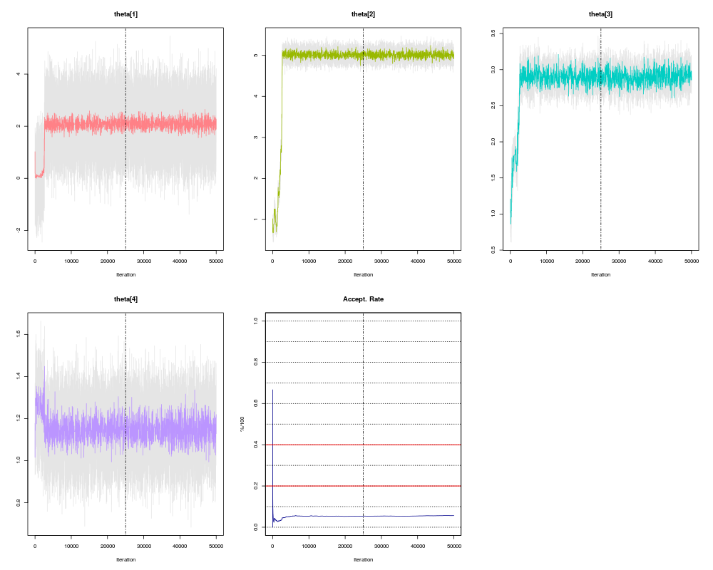
>   m1 <- GQD.mcmc(Xt,time,mesh=mesh.points,theta=theta.start,sds=proposal.sds,
+                  updates=updates)
Compiling C++ code. Please wait.                                                                                                           
 ================================================================
                  Generalized Ornstein-Uhlenbeck                 
 ================================================================
 _____________________ Drift Coefficients _______________________
 G0 : theta[1]*(theta[2]+theta[3]*sin(0.25*pi*t))                
 G1 : -theta[1]                                                  
 G2                                                              
 ___________________ Diffusion Coefficients _____________________
 Q0 : theta[4]*theta[4]                                          
 Q1                                                              
 Q2                                                              
 _____________________ Prior Distributions ______________________
                                                                 
 d(theta):dnorm(theta[1],5,5)                                    
=================================================================
                                                                 
 _______________________ Model/Chain Info _______________________
 Chain Updates       : 50000                                     
 Burned Updates      : 25000                                     
 Time Homogeneous    : No                                        
 Data Resolution     : Homogeneous: dt=0.25                      
 # Removed Transits. : None                                      
 Density approx.     : Normally distributed diffusion.           
 Elapsed time        : 00:00:56                                  
 ...   ...   ...   ...   ...   ...   ...   ...   ...   ...   ... 
 dim(theta)          : 4                                         
 DIC                 : 501.283                                   
 pd (eff. dim(theta)): 4.069                                     
 ----------------------------------------------------------------
> 
>  
>  #------------------------------------------------------------------------------
>  # Define coefficients of model 2
>  #------------------------------------------------------------------------------
> 
>   GQD.remove()
[1] "Removed :  G0 G1 Q0 priors"
>   G0 <- function(t){theta[1]*(theta[2]+theta[3]*sin(0.25*pi*t))}
>   G1 <- function(t){-theta[1]}
>   Q1 <- function(t){theta[4]*theta[4]}
> 
>   proposal.sds  <-  c(0.8,0.1,0.1,0.1)
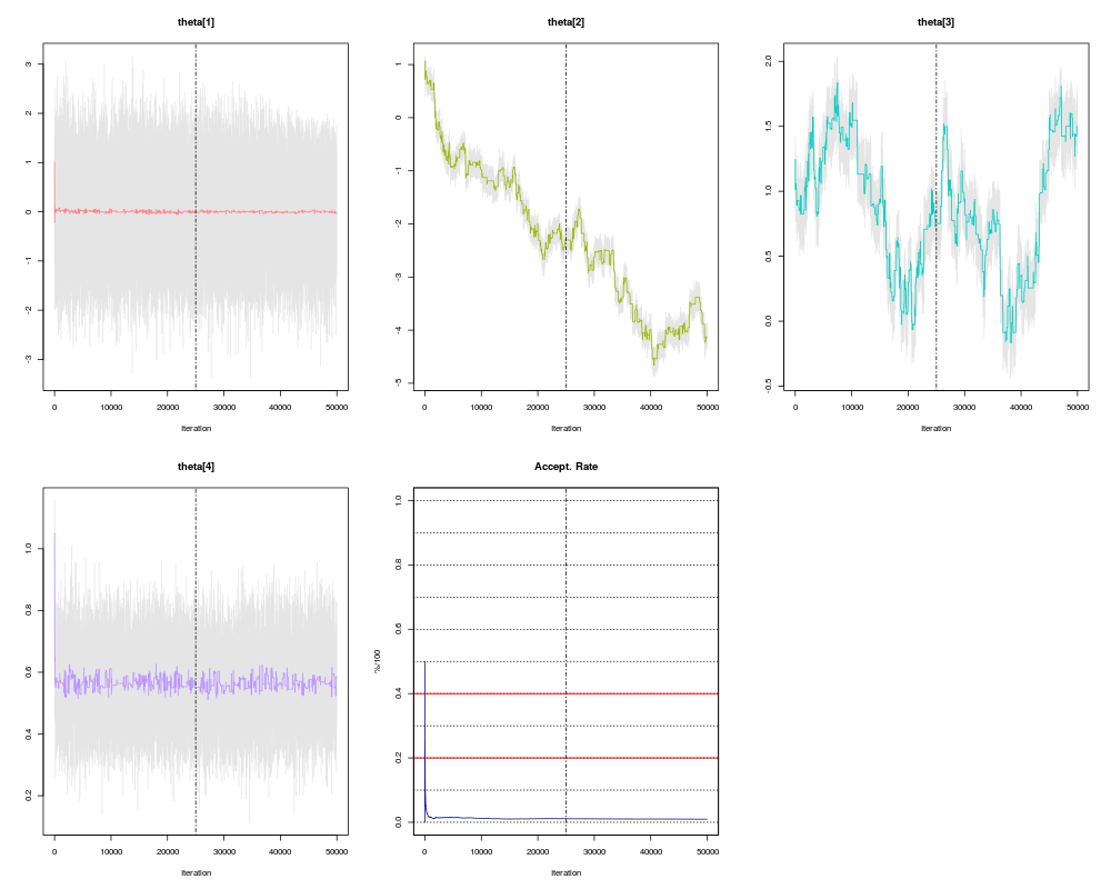
>   m2 <- GQD.mcmc(Xt,time,mesh=mesh.points,theta=theta.start,sds=proposal.sds,
+                  updates=updates)
Compiling C++ code. Please wait.                                                                                                           
 ================================================================
                  Generalized Quadratic Diffusion (GQD)          
 ================================================================
 _____________________ Drift Coefficients _______________________
 G0 : theta[1]*(theta[2]+theta[3]*sin(0.25*pi*t))                
 G1 : -theta[1]                                                  
 G2                                                              
 ___________________ Diffusion Coefficients _____________________
 Q0                                                              
 Q1 : theta[4]*theta[4]                                          
 Q2                                                              
 _____________________ Prior Distributions ______________________
                                                                 
 d(theta):None.                                                  
=================================================================
                                                                       
 _______________________ Model/Chain Info _______________________      
 Chain Updates       : 50000                                           
 Burned Updates      : 25000                                           
 Time Homogeneous    : No                                              
 Data Resolution     : Homogeneous: dt=0.25                            
 # Removed Transits. : None                                            
 Density approx.     : 4 Ord. Truncation +4th Ord. Saddlepoint Appr.   
 Elapsed time        : 00:01:02                                        
 ...   ...   ...   ...   ...   ...   ...   ...   ...   ...   ...       
 dim(theta)          : 4                                               
 DIC                 : 458.293                                         
 pd (eff. dim(theta)): 4.063                                           
 ----------------------------------------------------------------      
> 
>   # Checkthe parameter estimates:
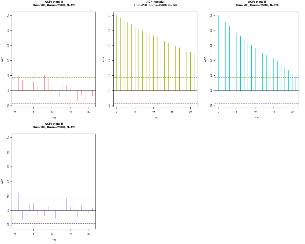
>   GQD.estimates(m2,thin = 200)
         Estimate Lower_CI Upper_CI
theta[1]    2.018    1.821    2.256
theta[2]    5.013    4.922    5.105
theta[3]    2.928    2.782    3.052
theta[4]    0.497    0.466    0.530
>  #------------------------------------------------------------------------------
>  # Summarize the output from the models.
>  #------------------------------------------------------------------------------
> 
>  GQD.dic(list(m1,m2))
        Elapsed_Time Time_Homogeneous       p          DIC      pD   N
Model 1     00:00:56               No   4.000      501.280   4.070 401
Model 2     00:01:02               No   4.000  [=] 458.290   4.060 401
>  
> #===============================================================================
> ## End(No test)
> 
> 
> 
> 
> 
> dev.off()
null device 
          1 
>