R Graphical Manual

Browse All

Last data update: 2014.03.03

R: MCMC Inference on Generalized Quadratic Diffusion Models...

GQD.mcmc

R Documentation

MCMC Inference on Generalized Quadratic Diffusion Models (GQDs).

Description

GQD.mcmc() uses parametrised coefficients (provided by the user as R-functions) to construct a C++ program in real time that allows the user to perform Bayesian inference on the resulting jump diffusion model. Given a set of starting parameters, a MCMC chain is returned for further analysis.

GQD.mcmc() performs inference using the Metropolis-Hastings algorithm for jump diffusions of the form:

where

and

Usage

GQD.mcmc(X, time, mesh=10, theta, sds, updates, burns=min(round(updates/2),25000),
         Dtype='Saddle', Trunc=c(4,4), RK.order=4, P=200, alpha=0,
         lower=min(na.omit(X))/2, upper=max(na.omit(X))*2,
         exclude=NULL, plot.chain=TRUE, Tag=NA, wrt=FALSE, print.output=TRUE)

Arguments

`X`	Time series (vector) of discretely observed points of the process of interest. These may be non-equidistant observations (see `time`).
`time`	A vector of time-stamps associated with each observation in `X`.
`mesh`	The number mesh points between any two given data points.
`theta`	The parameter vector of the process. `theta` are taken as the starting values of the MCMC chain and gives the dimension of the parameter vector used to calculate the DIC. Care should be taken to ensure that each element in `theta` is in fact used within the coefficient-functions, otherwise redundant parameters will be counted in the calculation of the DIC.
`sds`	Proposal distribution standard deviations. That is, for the i-th parameter the proposal distribution is ~ Normal(...,`sds`[i]^2)
`updates`	The number of chain updates (including burned updates) to perform.
`burns`	The number of updates to burn. That is, the first `burns` values are omitted from the inference, although the entire chain is returned.
`exclude`	Vector indicating which transitions to exclude from the analysis. Default = `NULL`.
`plot.chain`	If `TRUE` (default), a trace plot is made of the resulting MCMC chain (see details).
`RK.order`	The order of the Runge-Kutta solver used to approximate the trajectories of cumulants. Must be 4 or (default) 10.
`Dtype`	Character string indicating the type of density approximation (see details) to use. Types: `'Saddlepoint'`, `'Normal'`, `'Gamma'`, `'InvGamma'` and `'Beta'` are supported (default = `'Saddlepoint'`).
`Trunc`	Vector of length 2 containing the cumulant truncation order and the density truncation order respectively. May take on values 4, 6 and 8 with the constraint that `Trunc[1] >= Trunc[2]`. Default is `c(4,4)`.
`P`	Normalization parameter indicating the number of points to use when normalizing members of the Pearson system (see details)
`alpha`	Normalization parameter controlig the mesh concentration when normalizing members of the Pearson system (see details). Increasing `alpha` decreases concentration around the mean and vice versa (default `alpha = 0`).
`lower,upper`	Lower and upper bounds for the normalization range.
`Tag`	`Tag` can be used to name (tag) an MCMC run e.g. `Tag='Run_1'`
`wrt`	If `TRUE` a .cpp file will be written to the current directory. For bug report diagnostics.
`print.output`	If `TRUE` information about the model and algorithm is printed to the console.

Details

GQD.mcmc() operates by searching the workspace for functions with names that match the coefficients of the predefined stochastic differential equation. Only the required coefficients need to be specified e.g. G0(t),G1(t) and Q0(t) for an Ornstein-Uhlenbeck model. Unspecified coefficients are ignored. When a new model is to be defined, the current model may be removed from the workspace by using the GQD.remove function, after which the new coefficients may be supplied.

Value

`par.matrix`	A matrix containing the MCMC chain on `theta`.
`acceptence.rate`	A vector containing the acceptance rate of the MCMC at every iteration.
`model.info`	A list of variables pertaining to inference calculations.
`model.info$elapsed.time`	The runtime, in h/m/s format,of the MCMC procedure (excluding compile time).
`model.info$time.homogeneous`	‘No’ if the model has time-homogeneous coefficients and ‘Yes’ otherwise.
`model.info$p`	The dimension of `theta`.
`model.info$DIC`	Calculated Deviance Information Criterion.
`model.info$pd`	Effective number of parameters (see `model.info$DIC`).

Syntactical jargon

Synt. [1]: The coefficients of the GQD may be parameterized using the reserved variable theta. For example:

G0 <- function(t){theta[1]*(theta[2]+sin(2*pi*(t-theta[3])))}.

Synt. [2]: Due to syntactical differences between R and C++ special functions have to be used when terms that depend on t. When the function cannot be separated in to terms that contain a single t, the prod(a,b) function must be used. For example:

G0 <- function(t){0.1*(10+0.2*sin(2*pi*t)+0.3*prod(sqrt(t),1+cos(3*pi*t)))}.

Here sqrt(t)*cos(3*pi*t) constitutes the product of two terms that cannot be written i.t.o. a single t. To circumvent this isue, one may use the prod(a,b) function.

Synt. [3]: Similarly, the ^ - operator is not overloaded in C++. Instead the pow(x,p) function may be used to calculate x^p. For example sin(2*pi*t)^3 in:

G0 <- function(t){0.1*(10+0.2*pow(sin(2*pi*t),3))}.

Note

Note [1]: When plot.chain is TRUE, a trace plot is created of the resulting MCMC along with the acceptance rate at each update. This may save time when scrutinizing initial MCMC runs.

Author(s)

Etienne A.D. Pienaar: etiennead@gmail.com

References

Updates available on GitHub at https://github.com/eta21.

Daniels, H.E. 1954 Saddlepoint approximations in statistics. Ann. Math. Stat., 25:631–650.

Eddelbuettel, D. and Romain, F. 2011 Rcpp: Seamless R and C++ integration. Journal of Statistical Software, 40(8):1–18,. URL http://www.jstatsoft.org/v40/i08/.

Eddelbuettel, D. 2013 Seamless R and C++ Integration with Rcpp. New York: Springer. ISBN 978-1-4614-6867-7.

Eddelbuettel, D. and Sanderson, C. 2014 Rcpparmadillo: Accelerating R with high-performance C++ linear algebra. Computational Statistics and Data Analysis, 71:1054–1063. URL http://dx.doi.org/10.1016/j.csda.2013.02.005.

Feagin, T. 2007 A tenth-order Runge-Kutta method with error estimate. In Proceedings of the IAENG Conf. on Scientifc Computing.

Varughese, M.M. 2013 Parameter estimation for multivariate diffusion systems. Comput. Stat. Data An., 57:417–428.

Examples


#===============================================================================
# This example simulates a time inhomogeneous diffusion and shows how to conduct
# inference using GQD.mcmc
#-------------------------------------------------------------------------------
 data(SDEsim1)
 attach(SDEsim1)
 par(mfrow=c(1,1))
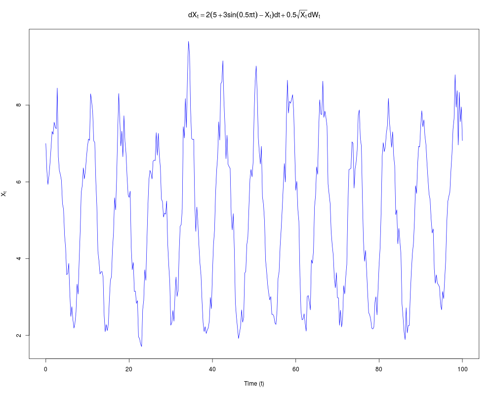
 expr1=expression(dX[t]==2*(5+3*sin(0.5*pi*t)-X[t])*dt+0.5*sqrt(X[t])*dW[t])
 plot(Xt~time,type='l',col='blue',xlab='Time (t)',ylab=expression(X[t]),main=expr1)
#------------------------------------------------------------------------------
# Define parameterized coefficients of the process, and set up starting
# parameters.
# True model: dX_t = 2X_t(5+3sin(0.25 pi t)-X_t)dt+0.5X_tdW_t
#------------------------------------------------------------------------------

# Remove any existing coeffients. If none are pressent NAs will be returned, but
# this is a safeguard against overlapping.
GQD.remove()

# Define time dependant coefficients. Note that all functions have a single argument.
# This argument has to be `t' in order for the dependancy to be recognized.
# theta does not have to be defined as an argument.

G0 <- function(t){theta[1]*(theta[2]+theta[3]*sin(0.25*pi*t))}
G1 <- function(t){-theta[1]}
Q1 <- function(t){theta[4]*theta[4]}

theta.start  <- c(1,1,1,1)                    # Starting values for the chain
proposal.sds <- c(0.4,0.3,0.2,0.1)*1/2        # Std devs for proposal distributions
mesh.points  <- 10                            # Number of mesh points
updates      <- 50000                         # Perform 50000 updates

#------------------------------------------------------------------------------
# Run the MCMC procedure for the model defined above
#------------------------------------------------------------------------------

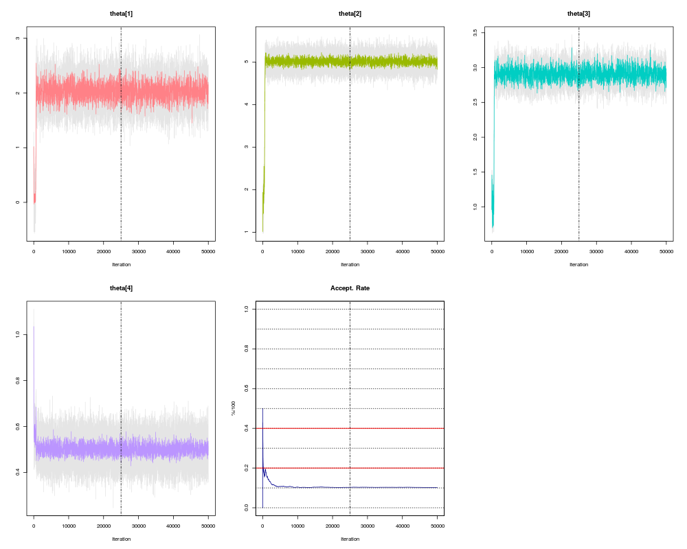
m1 <- GQD.mcmc(Xt,time,mesh=mesh.points,theta=theta.start,sds=proposal.sds,
               updates=updates)

# Calculate estimates:
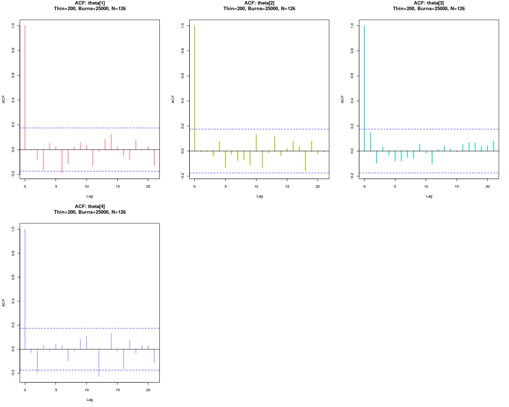
GQD.estimates(m1,thin=200)
#===============================================================================

Results


R version 3.3.1 (2016-06-21) -- "Bug in Your Hair"
Copyright (C) 2016 The R Foundation for Statistical Computing
Platform: x86_64-pc-linux-gnu (64-bit)

R is free software and comes with ABSOLUTELY NO WARRANTY.
You are welcome to redistribute it under certain conditions.
Type 'license()' or 'licence()' for distribution details.

R is a collaborative project with many contributors.
Type 'contributors()' for more information and
'citation()' on how to cite R or R packages in publications.

Type 'demo()' for some demos, 'help()' for on-line help, or
'help.start()' for an HTML browser interface to help.
Type 'q()' to quit R.

> library(DiffusionRgqd)
> png(filename="/home/ddbj/snapshot/RGM3/R_CC/result/DiffusionRgqd/GQD.mcmc.Rd_%03d_medium.png", width=480, height=480)
> ### Name: GQD.mcmc
> ### Title: MCMC Inference on Generalized Quadratic Diffusion Models (GQDs).
> ### Aliases: GQD.mcmc
> ### Keywords: syntax C++ mcmc
> 
> ### ** Examples
> 
> ## No test: 
> #===============================================================================
> # This example simulates a time inhomogeneous diffusion and shows how to conduct
> # inference using GQD.mcmc
> #-------------------------------------------------------------------------------
>  data(SDEsim1)
>  attach(SDEsim1)
>  par(mfrow=c(1,1))
>  expr1=expression(dX[t]==2*(5+3*sin(0.5*pi*t)-X[t])*dt+0.5*sqrt(X[t])*dW[t])
>  plot(Xt~time,type='l',col='blue',xlab='Time (t)',ylab=expression(X[t]),main=expr1)
> #------------------------------------------------------------------------------
> # Define parameterized coefficients of the process, and set up starting
> # parameters.
> # True model: dX_t = 2X_t(5+3sin(0.25 pi t)-X_t)dt+0.5X_tdW_t
> #------------------------------------------------------------------------------
> 
> # Remove any existing coeffients. If none are pressent NAs will be returned, but
> # this is a safeguard against overlapping.
> GQD.remove()
[1] "Removed :  NA "
> 
> # Define time dependant coefficients. Note that all functions have a single argument.
> # This argument has to be `t' in order for the dependancy to be recognized.
> # theta does not have to be defined as an argument.
> 
> G0 <- function(t){theta[1]*(theta[2]+theta[3]*sin(0.25*pi*t))}
> G1 <- function(t){-theta[1]}
> Q1 <- function(t){theta[4]*theta[4]}
> 
> theta.start  <- c(1,1,1,1)                    # Starting values for the chain
> proposal.sds <- c(0.4,0.3,0.2,0.1)*1/2        # Std devs for proposal distributions
> mesh.points  <- 10                            # Number of mesh points
> updates      <- 50000                         # Perform 50000 updates
> 
> #------------------------------------------------------------------------------
> # Run the MCMC procedure for the model defined above
> #------------------------------------------------------------------------------
> 
> m1 <- GQD.mcmc(Xt,time,mesh=mesh.points,theta=theta.start,sds=proposal.sds,
+                updates=updates)
Compiling C++ code. Please wait.                                                                                                           
 ================================================================
                  Generalized Quadratic Diffusion (GQD)          
 ================================================================
 _____________________ Drift Coefficients _______________________
 G0 : theta[1]*(theta[2]+theta[3]*sin(0.25*pi*t))                
 G1 : -theta[1]                                                  
 G2                                                              
 ___________________ Diffusion Coefficients _____________________
 Q0                                                              
 Q1 : theta[4]*theta[4]                                          
 Q2                                                              
 _____________________ Prior Distributions ______________________
                                                                 
 d(theta):None.                                                  
=================================================================
                                                                       
 _______________________ Model/Chain Info _______________________      
 Chain Updates       : 50000                                           
 Burned Updates      : 25000                                           
 Time Homogeneous    : No                                              
 Data Resolution     : Homogeneous: dt=0.25                            
 # Removed Transits. : None                                            
 Density approx.     : 4 Ord. Truncation +4th Ord. Saddlepoint Appr.   
 Elapsed time        : 00:01:31                                        
 ...   ...   ...   ...   ...   ...   ...   ...   ...   ...   ...       
 dim(theta)          : 4                                               
 DIC                 : 458.009                                         
 pd (eff. dim(theta)): 3.918                                           
 ----------------------------------------------------------------      
> 
> # Calculate estimates:
> GQD.estimates(m1,thin=200)
         Estimate Lower_CI Upper_CI
theta[1]    2.023    1.805    2.240
theta[2]    5.019    4.929    5.114
theta[3]    2.913    2.800    3.051
theta[4]    0.498    0.468    0.528
> #===============================================================================
> 
> ## End(No test)
> 
> 
> 
> 
> 
> dev.off()
null device 
          1 
>