Supported by Dr. Osamu Ogasawara and  . . |
|
Last data update: 2014.03.03 |
Calculate the First Passage Time Density of a Time-Homogeneous GQD Process to a Fixed Barrier.Description
dX_t = (theta[1]+theta[2]X_t+theta[3]X_t^2)dt+√{theta[4]+theta[5]X_t+theta[6]X_t^2}dW_t, to a fixed barrier. UsageGQD.passage(Xs, B, theta, t, delt) Arguments
Value
WarningWarning [1]: Some instability may occur when Warning [2]: The first passage time problem is considered from one side only i.e. Xs<B. For Xs>B one may equivalently consider Yt=-X_t, apply Ito's lemma and proceed as above. NoteNote [1]: Since time-homogeneity is assumed for the present implementation, the interface of Author(s)Etienne A.D. Pienaar: etiannead@gmail.com ReferencesUpdates available on GitHub at https://github.com/eta21. A. Buonocore, A. Nobile, and L. Ricciardi. 1987 A new integral equation for the evaluation of first-passage- time probability densities. Adv. Appl. Probab. 19:784–800. Daniels, H.E. 1954 Saddlepoint approximations in statistics. Ann. Math. Stat., 25:631–650. Eddelbuettel, D. and Romain, F. 2011 Rcpp: Seamless R and C++ integration. Journal of Statistical Software, 40(8):1–18,. URL http://www.jstatsoft.org/v40/i08/. Eddelbuettel, D. 2013 Seamless R and C++ Integration with Rcpp. New York: Springer. ISBN 978-1-4614-6867-7. Eddelbuettel, D. and Sanderson, C. 2014 Rcpparmadillo: Accelerating r with high-performance C++ linear algebra. Computational Statistics and Data Analysis, 71:1054–1063. URL http://dx.doi.org/10.1016/j.csda.2013.02.005. Feagin, T. 2007 A tenth-order Runge-Kutta method with error estimate. In Proceedings of the IAENG Conf. on Scientific Computing. R. G. Jaimez, P. R. Roman and F. T. Ruiz. 1995 A note on the volterra integral equation for the first-passage-time probability density. Journal of applied probability, 635–648. Varughese, M.M. 2013 Parameter estimation for multivariate diffusion systems. Comput. Stat. Data An., 57:417–428. See Also
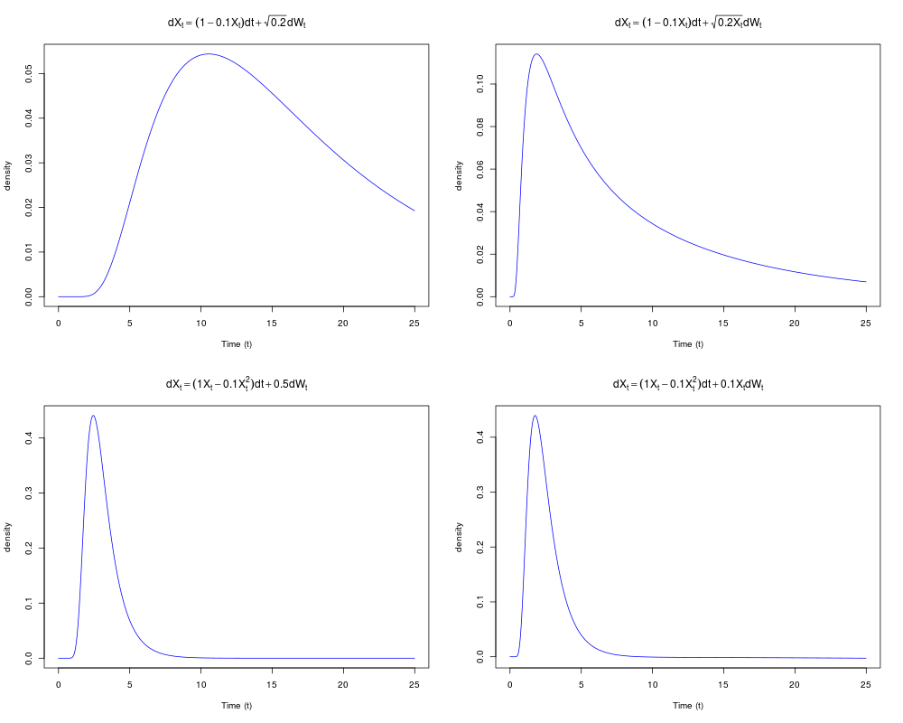
Examples#=============================================================================== # Calculate the first passage time from state X_0 = 7 to X_T =10 for # various diffusions, with T the first passage time. #=============================================================================== res1 <- GQD.passage(7,10,c(0.1*10,-0.1,0,0.2,0,0),25,1/100) res2 <- GQD.passage(7,10,c(0.1*10,-0.1,0,0,0.2,0),25,1/100) res3 <- GQD.passage(7,10,c(0,0.1*10,-0.1,0.5^2,0,0),25,1/100) res4 <- GQD.passage(7,10,c(0,0.1*10,-0.1,0,0,0.1^2),25,1/100) expr1 <- expression(dX[t]==(1-0.1*X[t])*dt+sqrt(0.2)*dW[t]) expr2 <- expression(dX[t]==(1-0.1*X[t])*dt+sqrt(0.2*X[t])*dW[t]) expr3 <- expression(dX[t]==(1*X[t]-0.1*X[t]^2)*dt+0.5*dW[t]) expr4 <- expression(dX[t]==(1*X[t]-0.1*X[t]^2)*dt+0.1*X[t]*dW[t]) #=============================================================================== # Plot the resulting first passage time densities. #=============================================================================== par(mfrow=c(2,2)) plot(res1$density~res1$time,type='l',main=expr1,xlab='Time (t)',ylab='density',col='blue') plot(res2$density~res2$time,type='l',main=expr2,xlab='Time (t)',ylab='density',col='blue') plot(res3$density~res3$time,type='l',main=expr3,xlab='Time (t)',ylab='density',col='blue') plot(res4$density~res4$time,type='l',main=expr4,xlab='Time (t)',ylab='density',col='blue') Results
R version 3.3.1 (2016-06-21) -- "Bug in Your Hair"
Copyright (C) 2016 The R Foundation for Statistical Computing
Platform: x86_64-pc-linux-gnu (64-bit)

R is free software and comes with ABSOLUTELY NO WARRANTY.
You are welcome to redistribute it under certain conditions.
Type 'license()' or 'licence()' for distribution details.

R is a collaborative project with many contributors.
Type 'contributors()' for more information and
'citation()' on how to cite R or R packages in publications.

Type 'demo()' for some demos, 'help()' for on-line help, or
'help.start()' for an HTML browser interface to help.
Type 'q()' to quit R.

> library(DiffusionRgqd)
> png(filename="/home/ddbj/snapshot/RGM3/R_CC/result/DiffusionRgqd/GQD.passage.Rd_%03d_medium.png", width=480, height=480)
> ### Name: GQD.passage
> ### Title: Calculate the First Passage Time Density of a Time-Homogeneous
> ###   GQD Process to a Fixed Barrier.
> ### Aliases: GQD.passage
> ### Keywords: syntax C++ first passage time
>
> ### ** Examples
>
> ## No test:
> #===============================================================================
> # Calculate the first passage time from state X_0 = 7 to X_T =10 for
> # various diffusions, with T the first passage time.
> #===============================================================================
>
>   res1 <- GQD.passage(7,10,c(0.1*10,-0.1,0,0.2,0,0),25,1/100)
Compiling C++ code. Please wait.                                          >   res2 <- GQD.passage(7,10,c(0.1*10,-0.1,0,0,0.2,0),25,1/100)
Compiling C++ code. Please wait.                                          >   res3 <- GQD.passage(7,10,c(0,0.1*10,-0.1,0.5^2,0,0),25,1/100)
Compiling C++ code. Please wait.                                          >   res4 <- GQD.passage(7,10,c(0,0.1*10,-0.1,0,0,0.1^2),25,1/100)
Compiling C++ code. Please wait.                                          >
>   expr1 <- expression(dX[t]==(1-0.1*X[t])*dt+sqrt(0.2)*dW[t])
>   expr2 <- expression(dX[t]==(1-0.1*X[t])*dt+sqrt(0.2*X[t])*dW[t])
>   expr3 <- expression(dX[t]==(1*X[t]-0.1*X[t]^2)*dt+0.5*dW[t])
>   expr4 <- expression(dX[t]==(1*X[t]-0.1*X[t]^2)*dt+0.1*X[t]*dW[t])
>
>
> #===============================================================================
> # Plot the resulting first passage time densities.
> #===============================================================================
>
>   par(mfrow=c(2,2))
>   plot(res1$density~res1$time,type='l',main=expr1,xlab='Time (t)',ylab='density',col='blue')
>   plot(res2$density~res2$time,type='l',main=expr2,xlab='Time (t)',ylab='density',col='blue')
>   plot(res3$density~res3$time,type='l',main=expr3,xlab='Time (t)',ylab='density',col='blue')
>   plot(res4$density~res4$time,type='l',main=expr4,xlab='Time (t)',ylab='density',col='blue')
>
> ## End(No test)
>
>
>
>
>
> dev.off()
null device
          1
>
|