Supported by Dr. Osamu Ogasawara and  . . |
|
Last data update: 2014.03.03 |
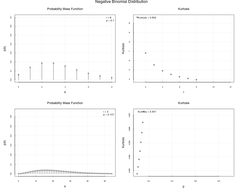
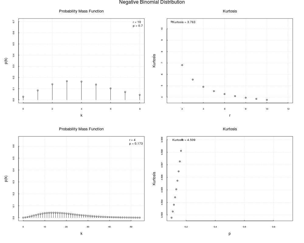
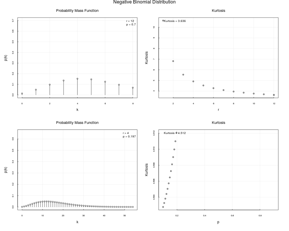
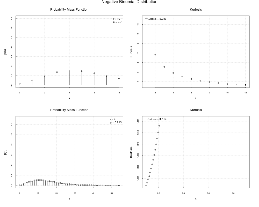
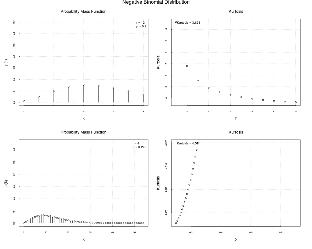
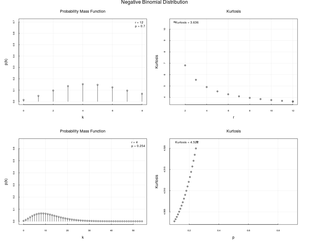
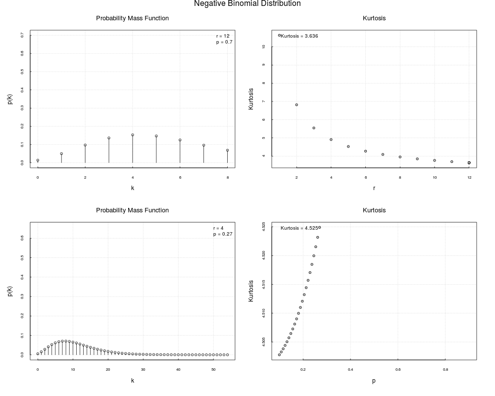
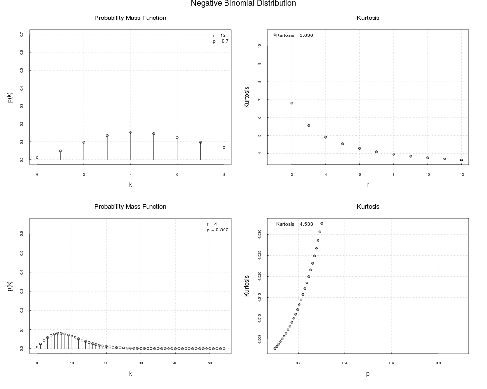
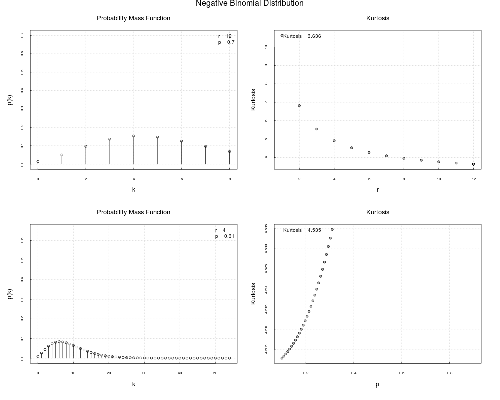
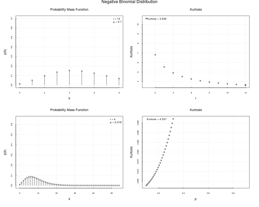
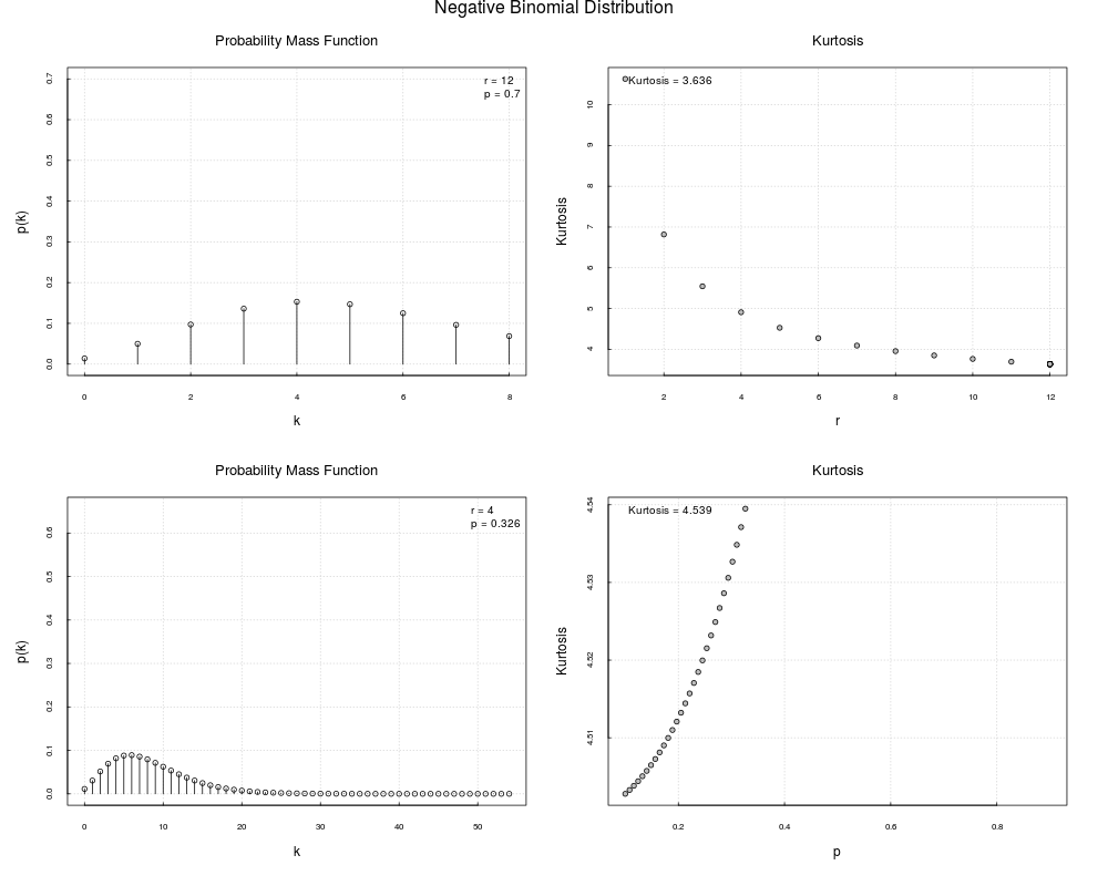
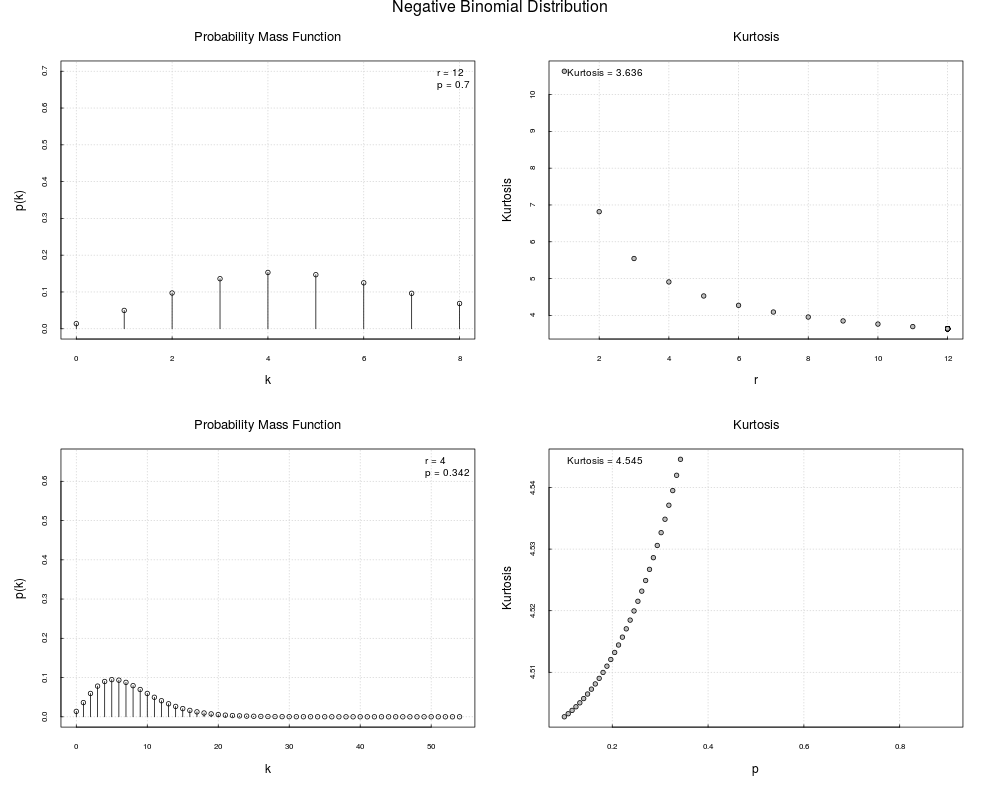
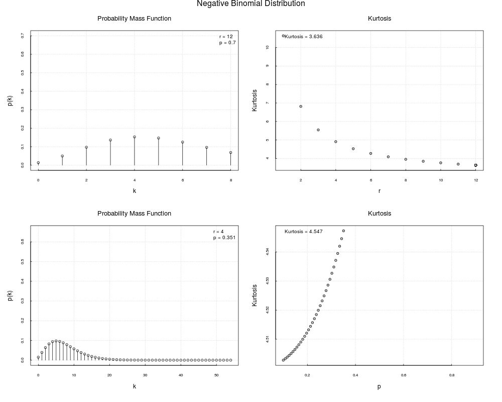
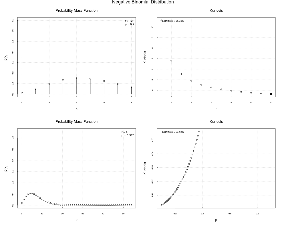
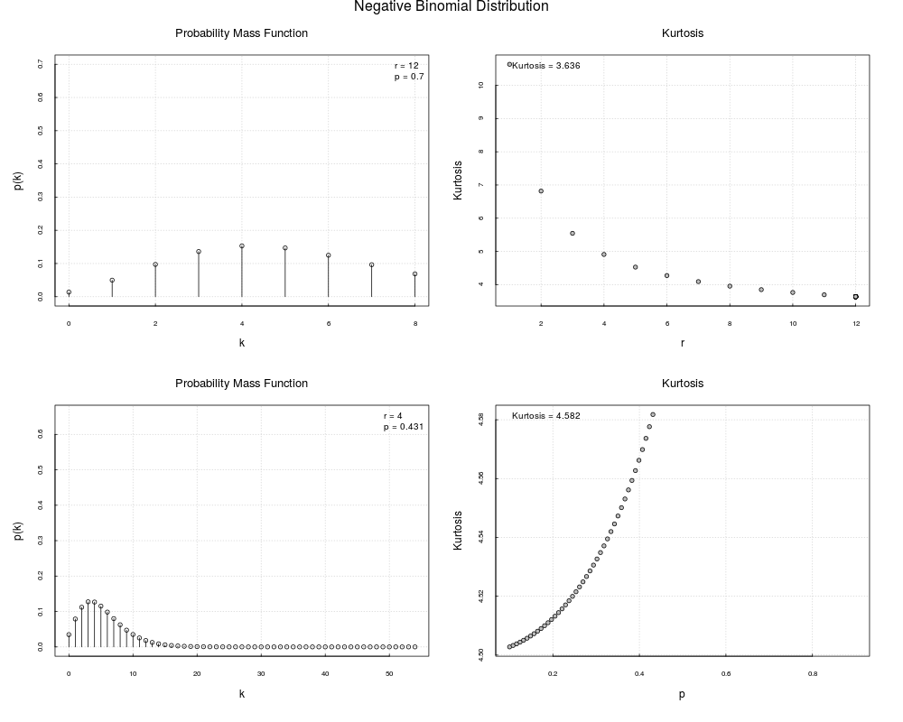
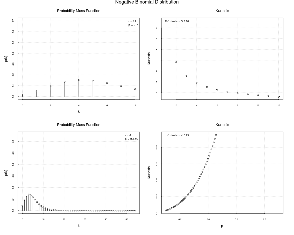
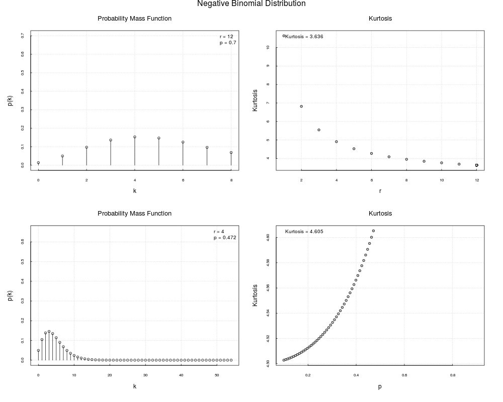
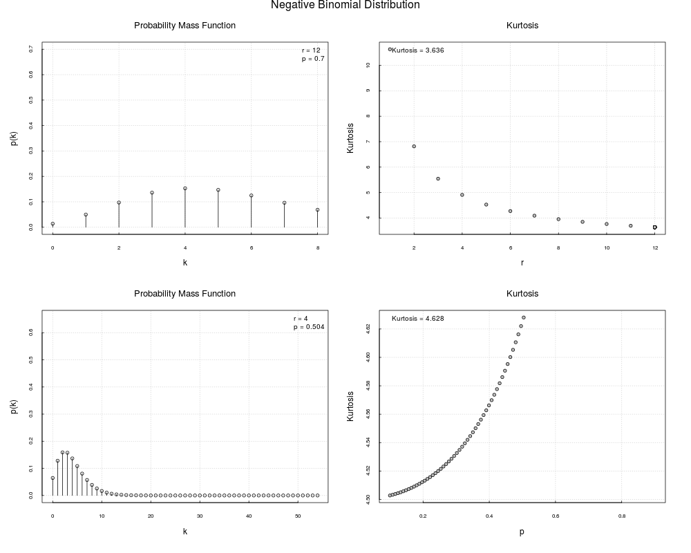
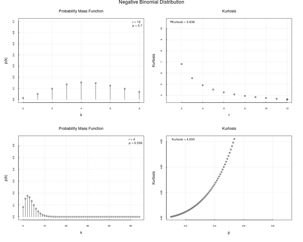
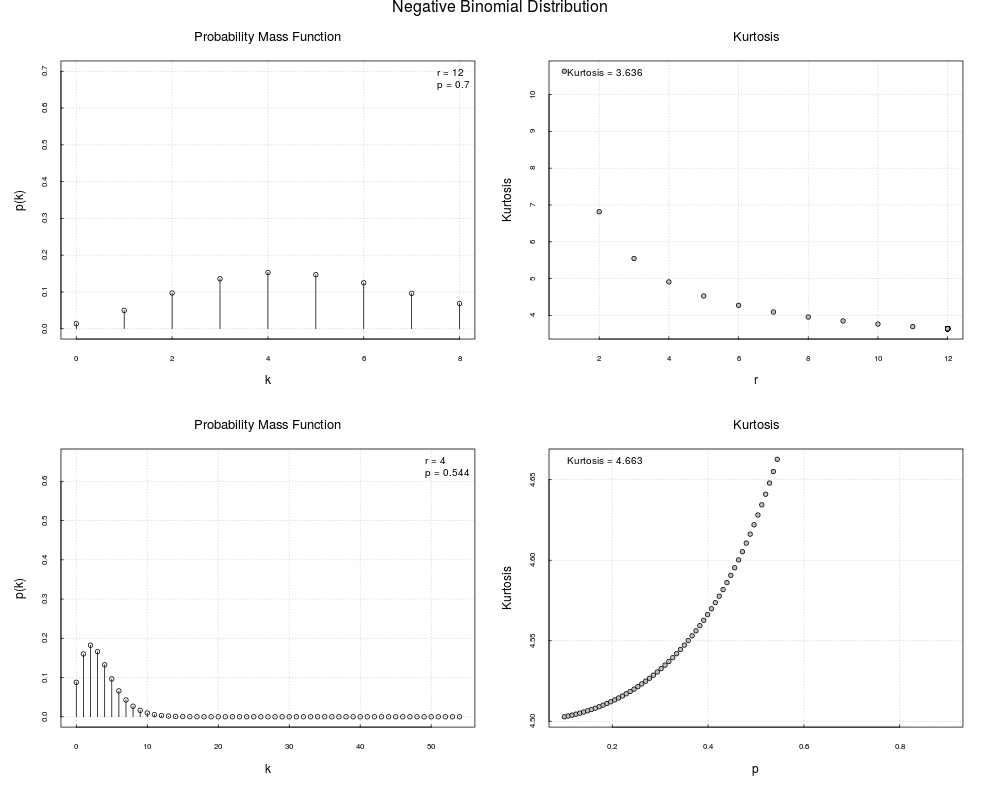
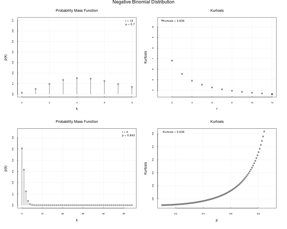
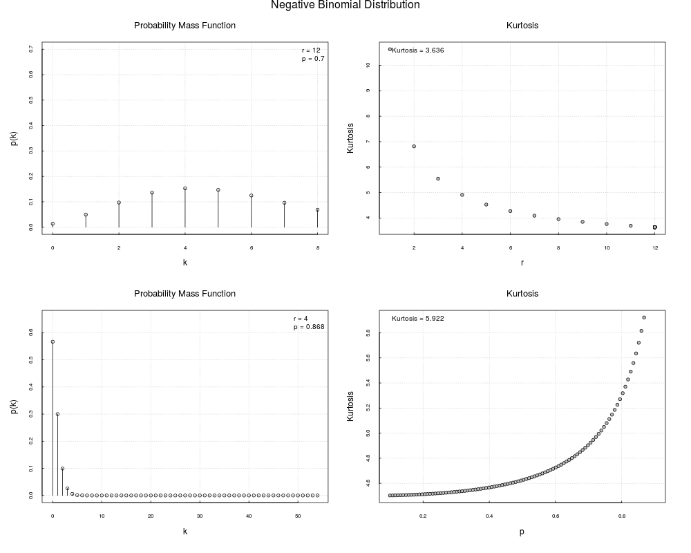
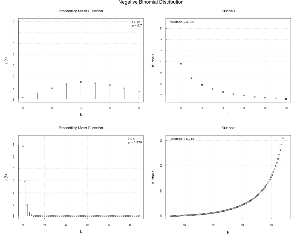
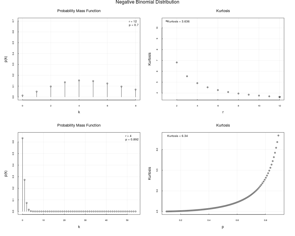
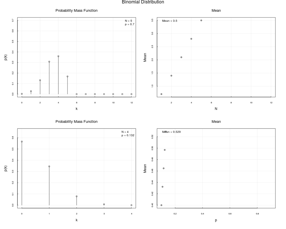
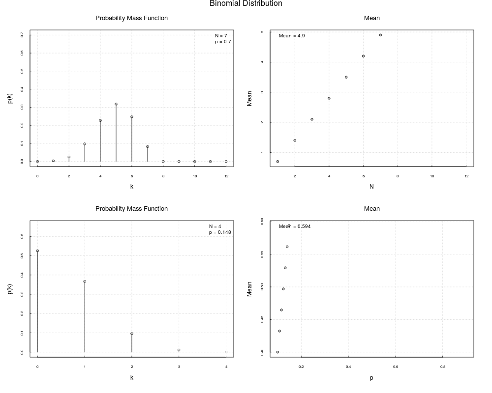
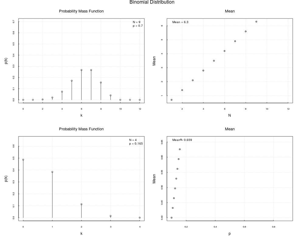
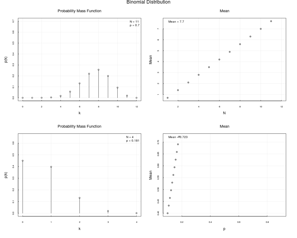
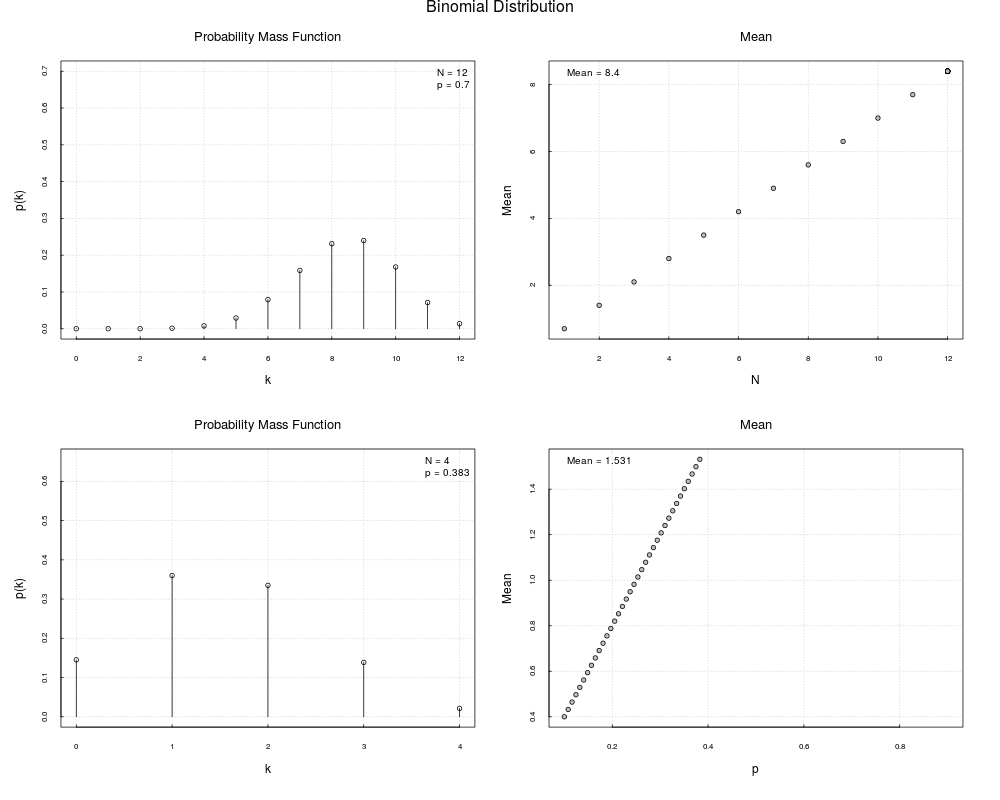
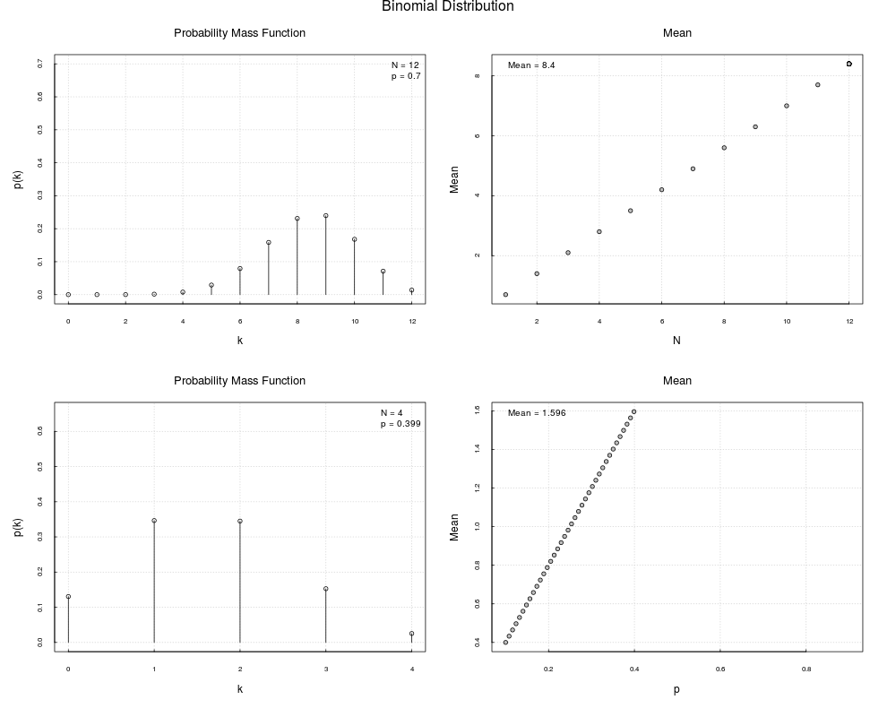
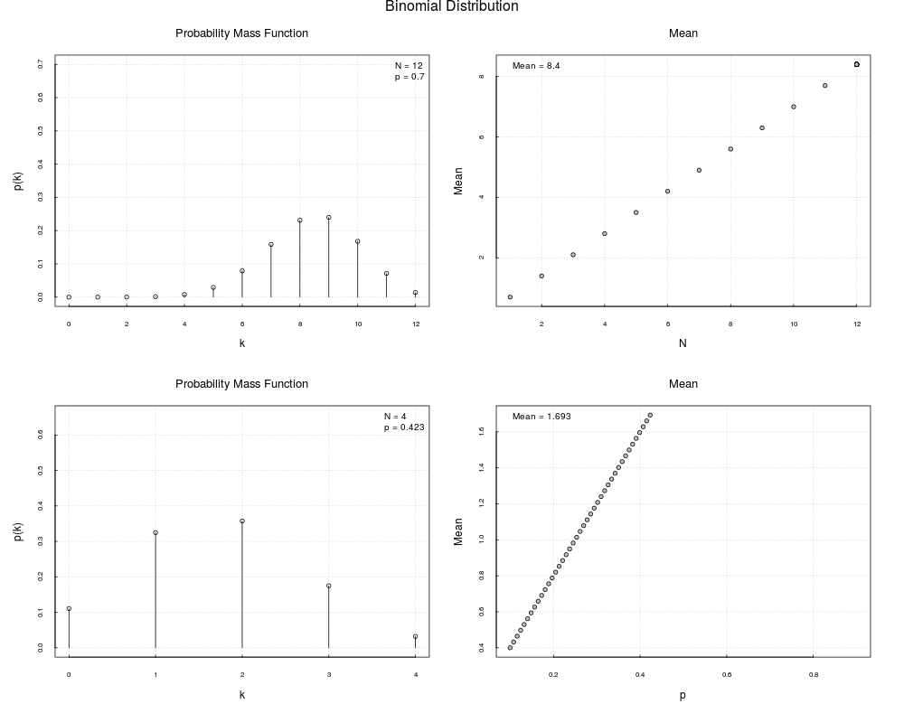
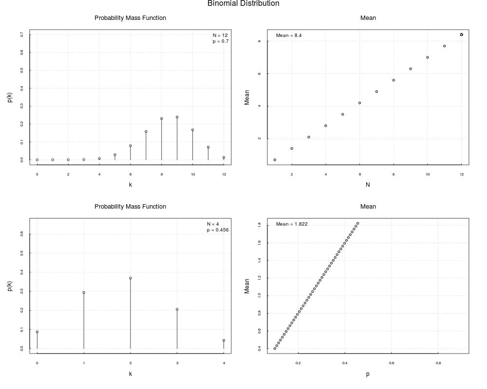
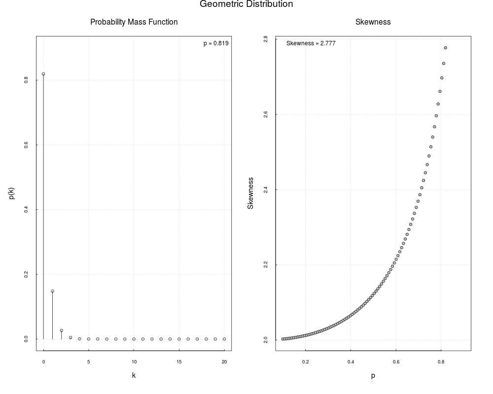
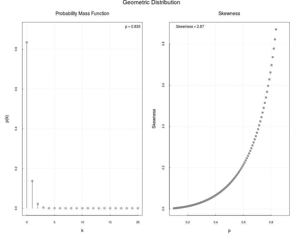
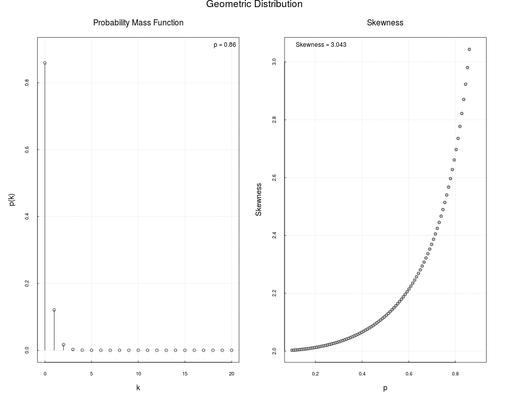
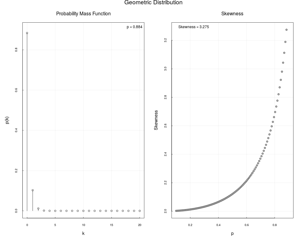
Dynamically Visualized Discrete Probability Distributions and Their MomentsDescriptionThis function is aimed at dynamically visualizing discrete probability distributions and their moments when the parameters changed. UsageDynDis(name, par_matrix, total = c(100, 100, 100), choice = "cdf", interval = 0.05, const_par = c(NULL, NULL, NULL)) Arguments
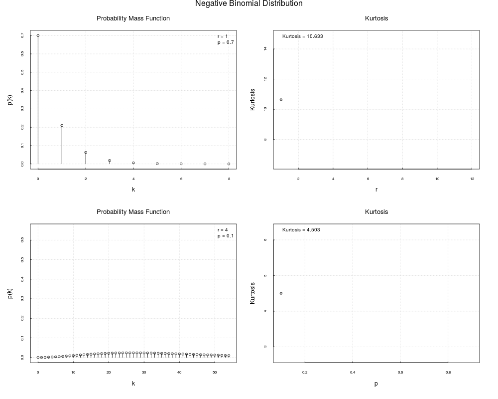
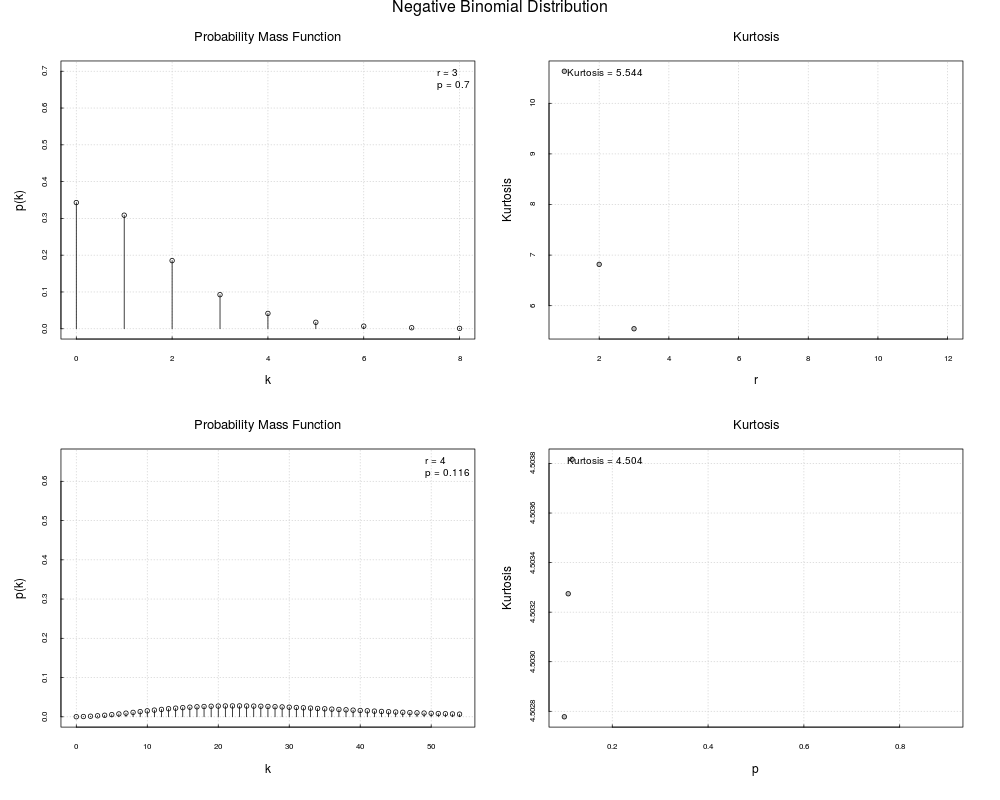
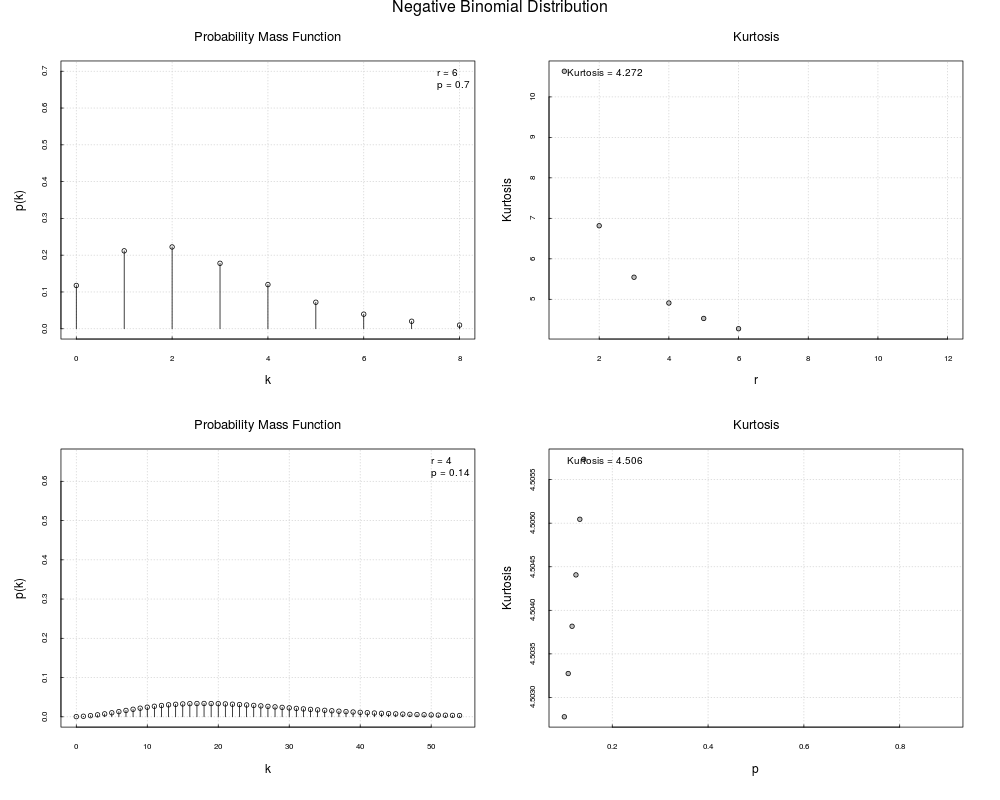
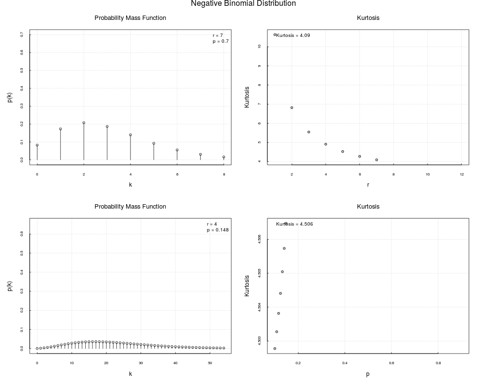
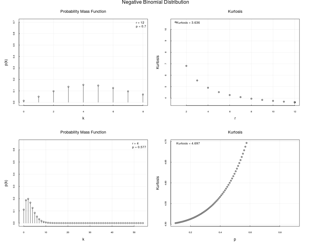
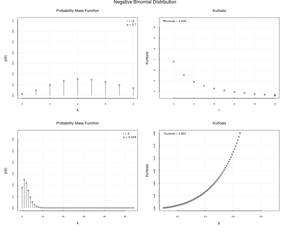
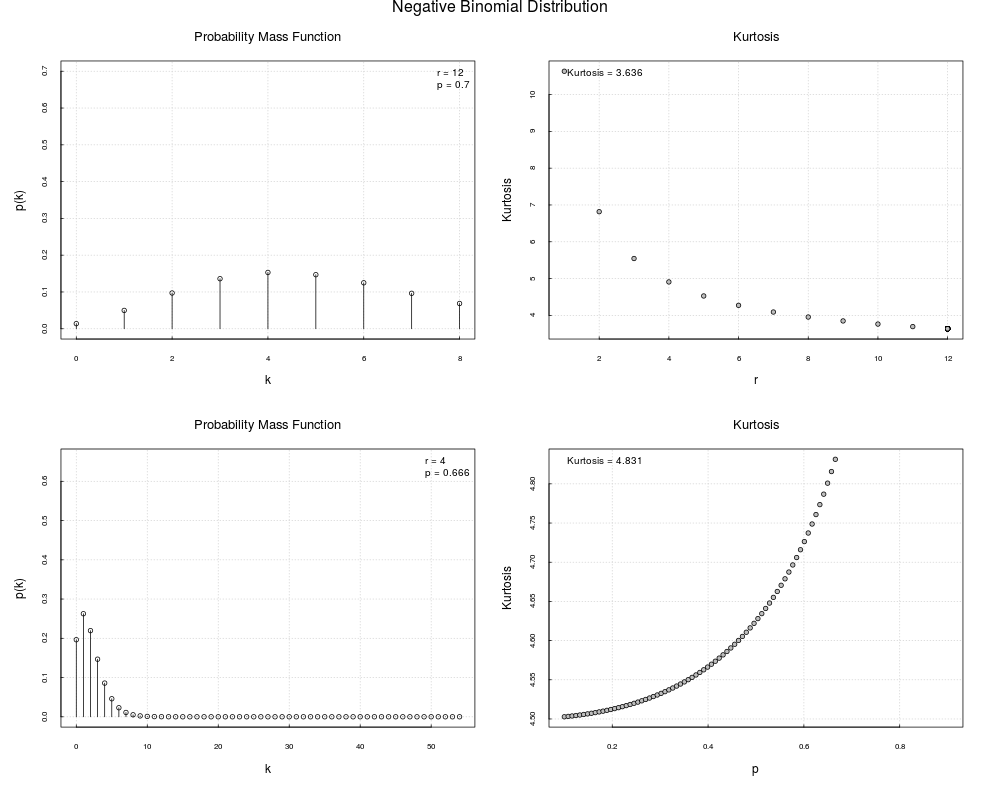
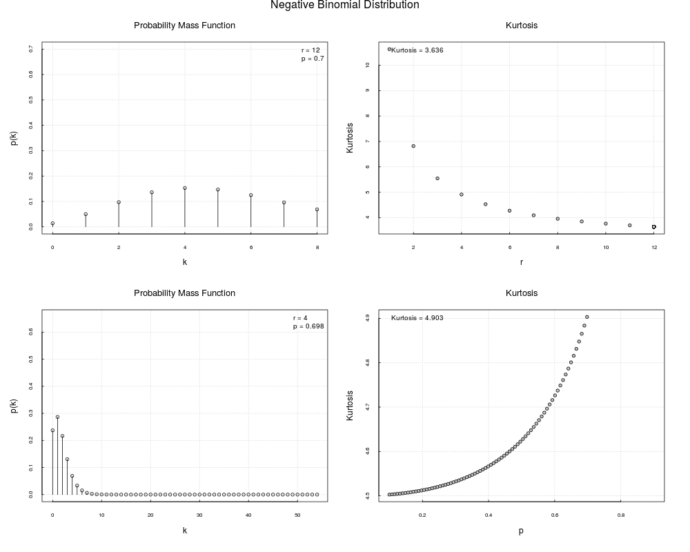
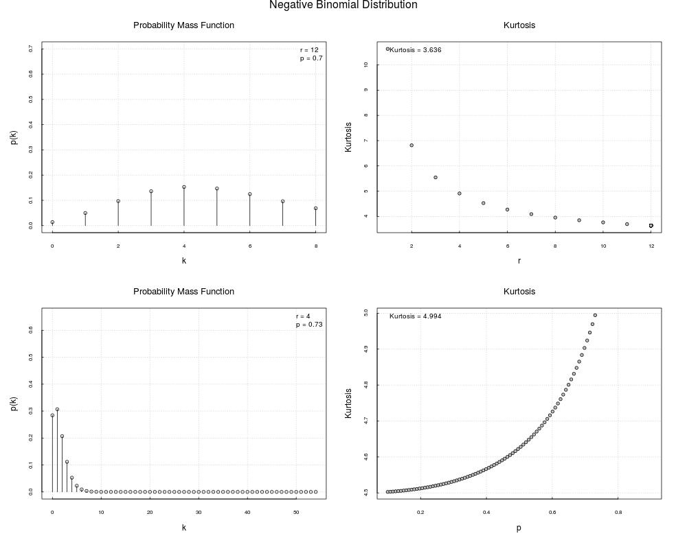
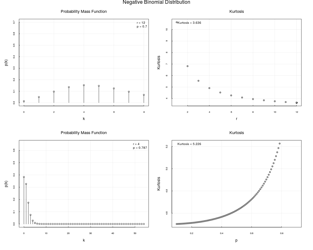
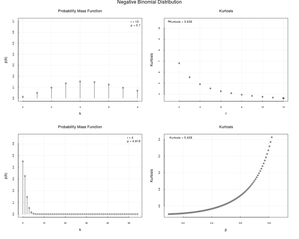
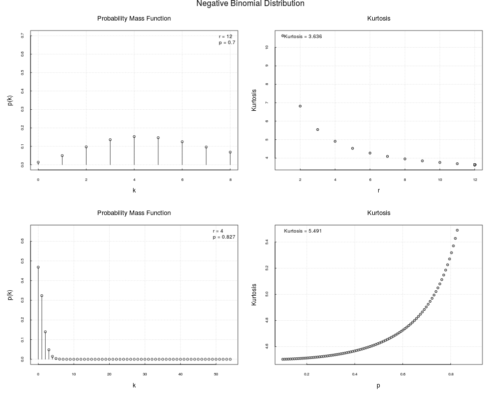
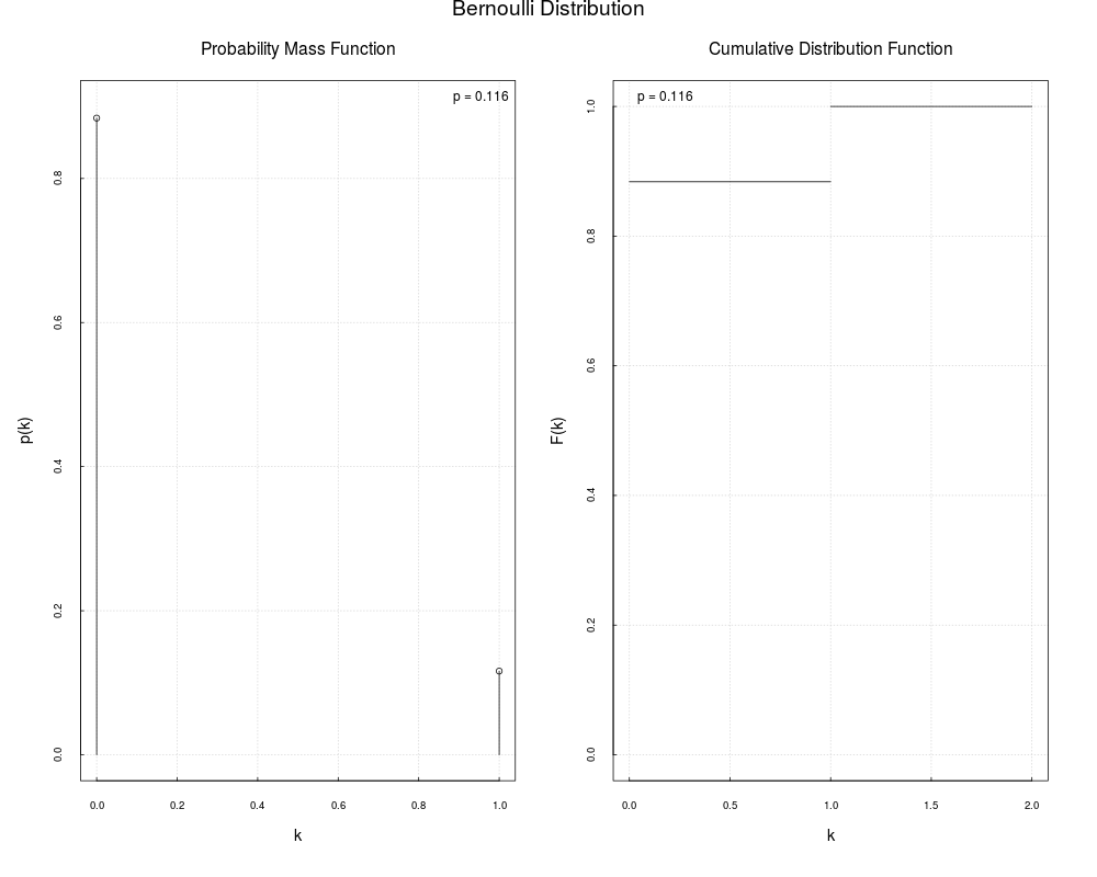
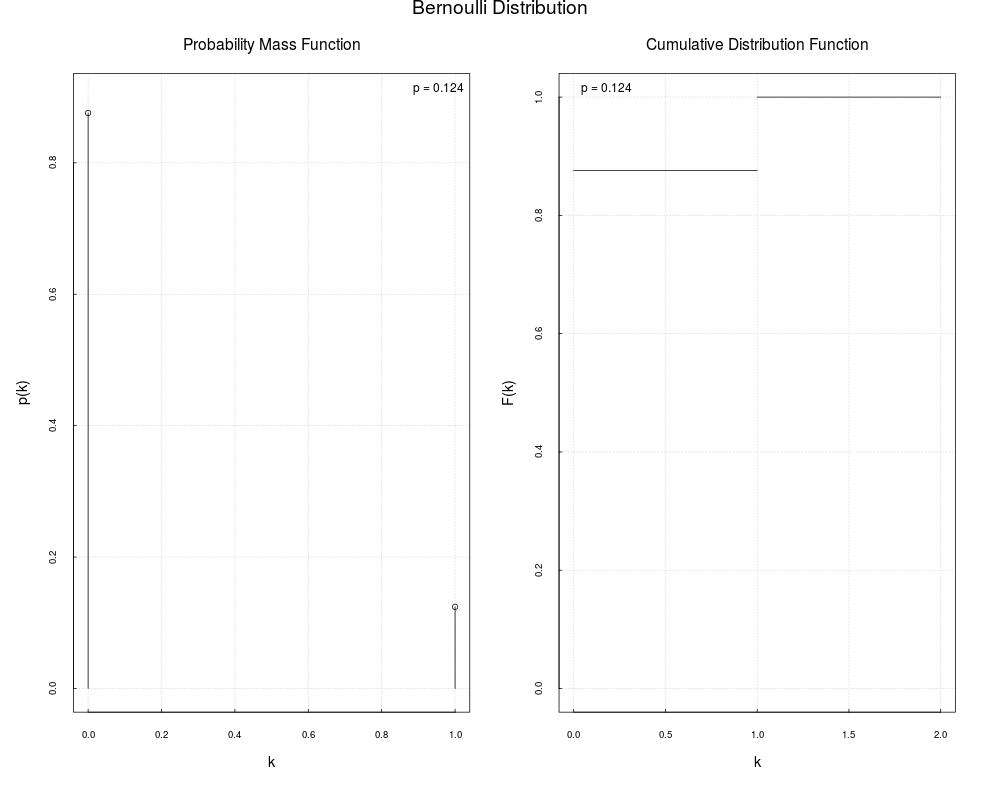
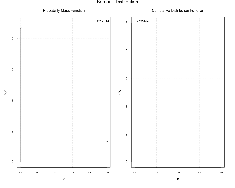
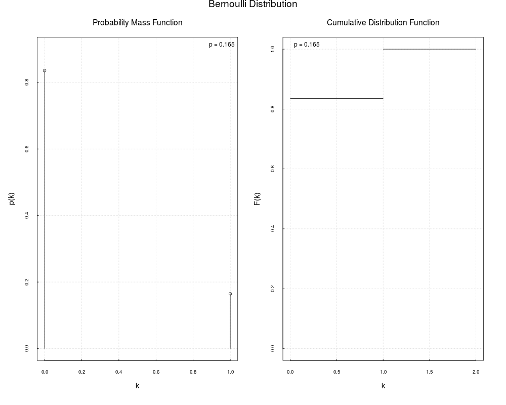
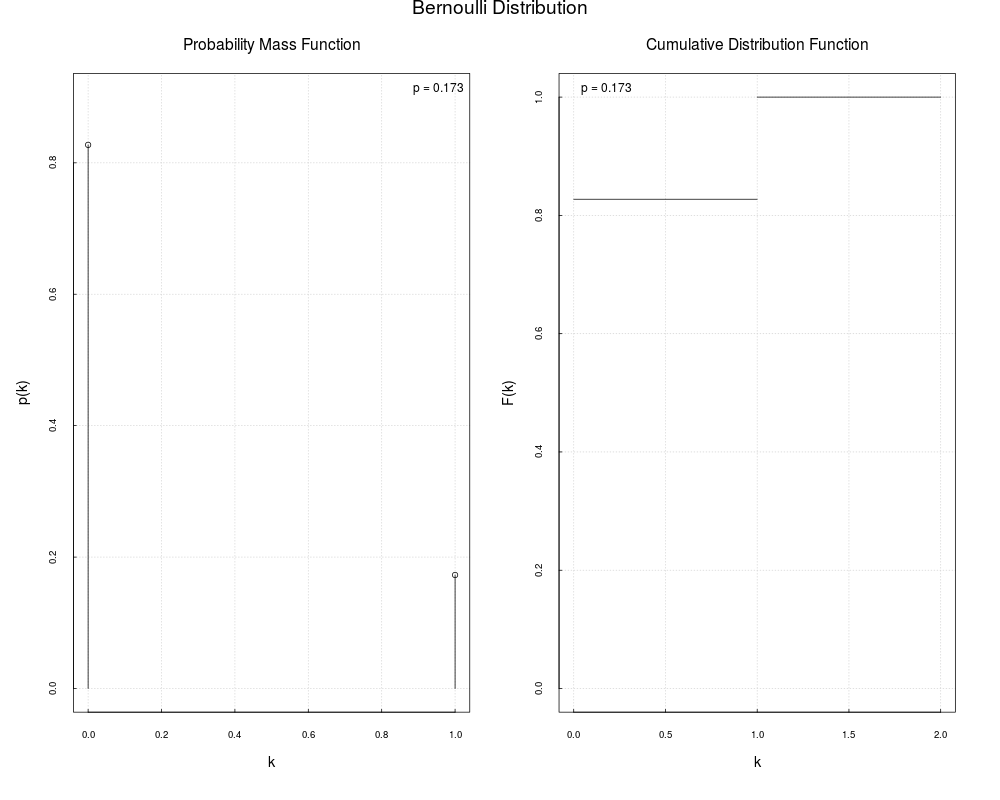
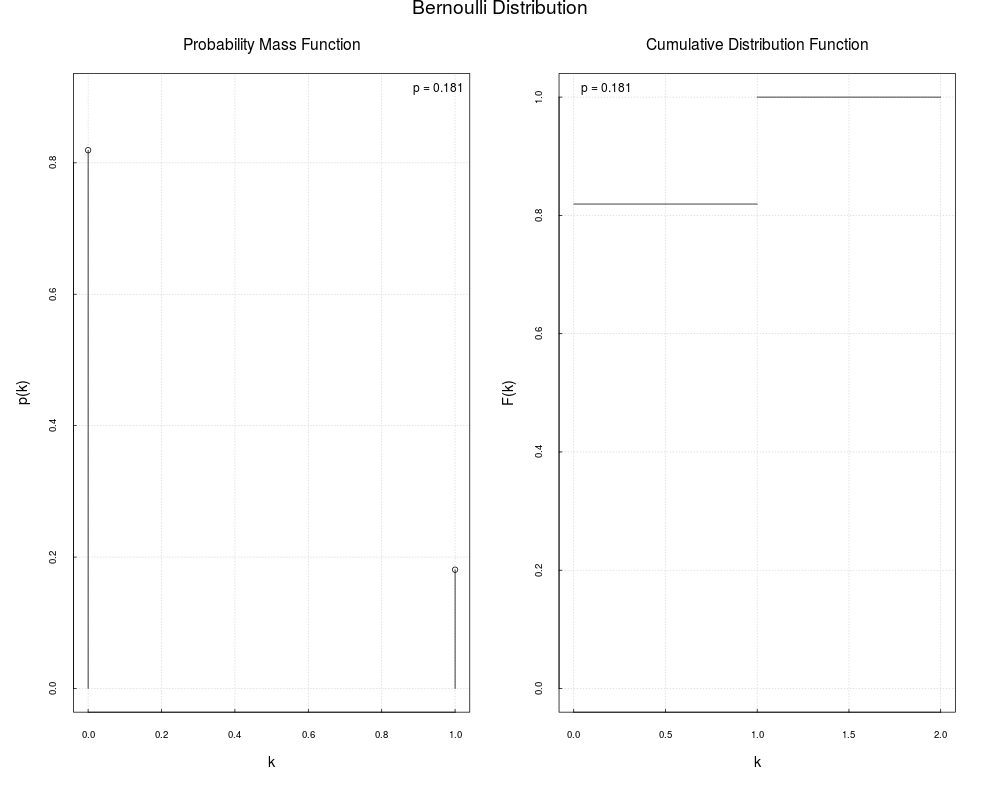
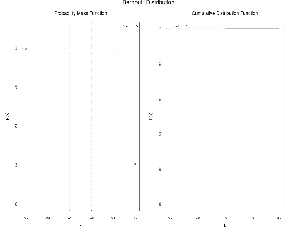
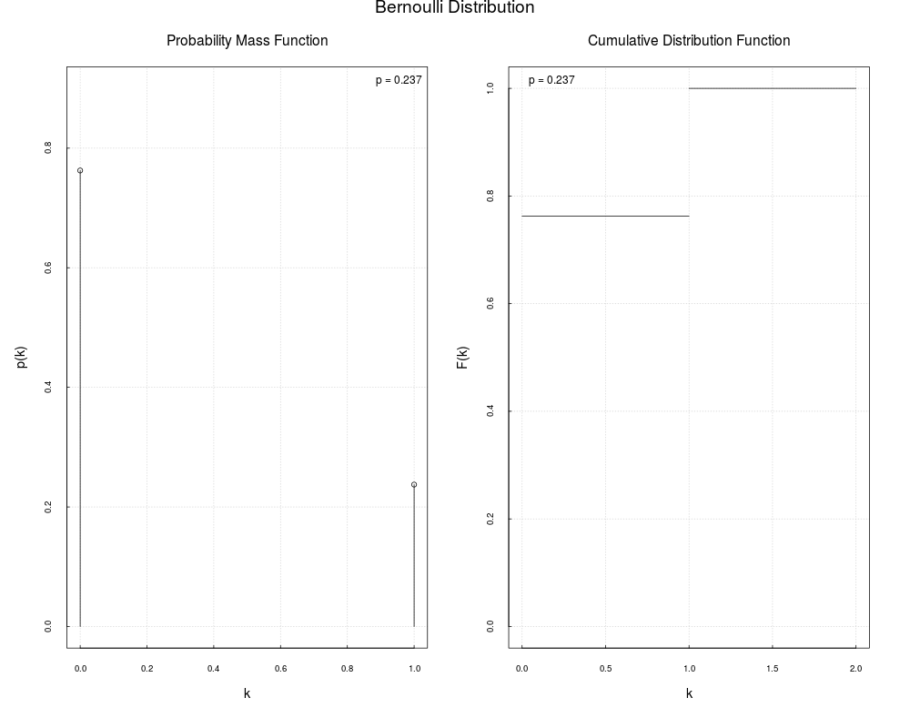
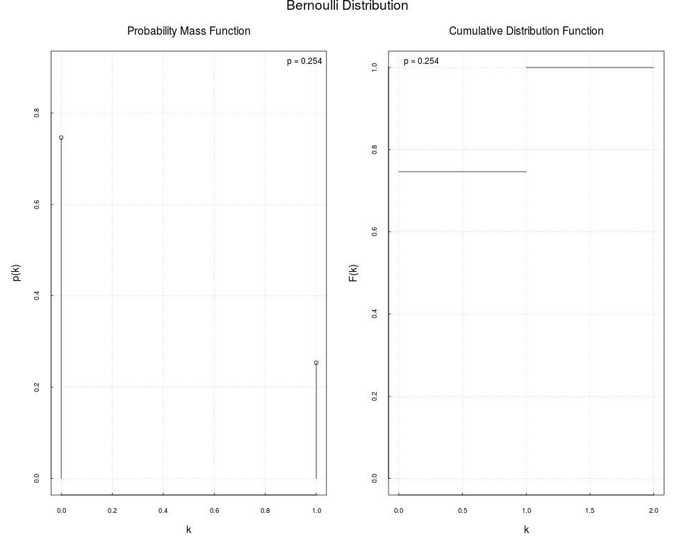
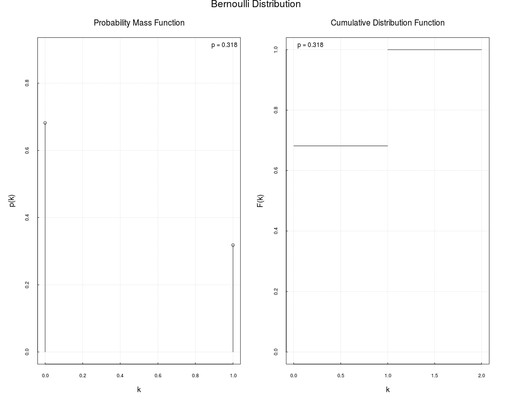
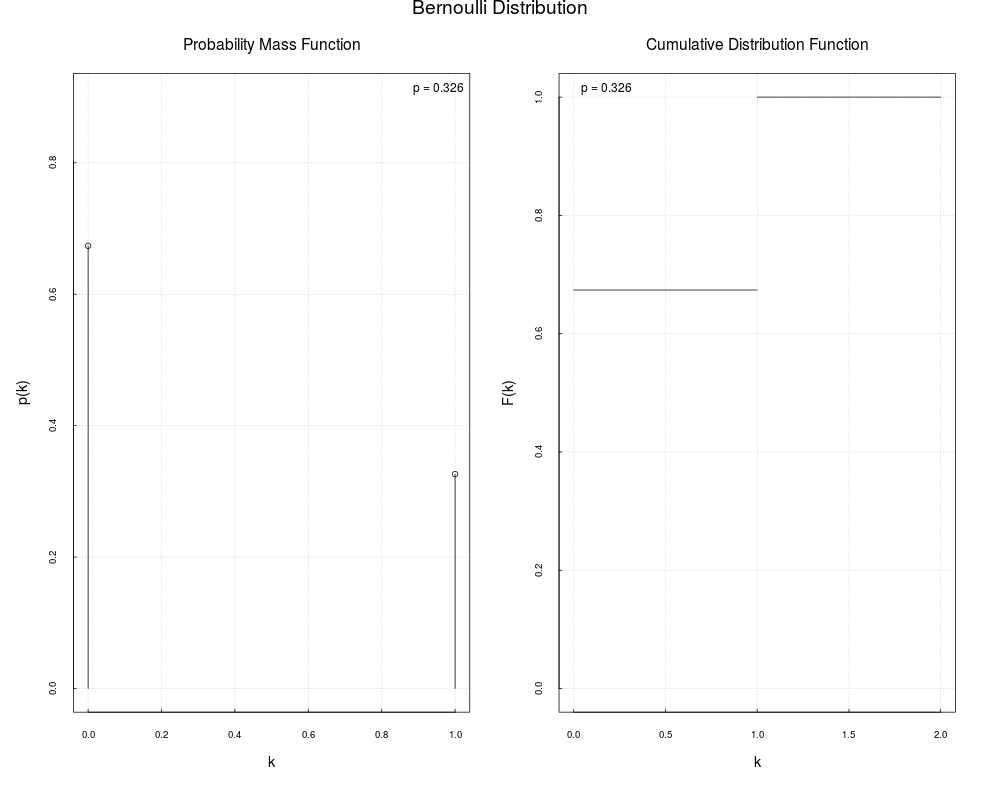
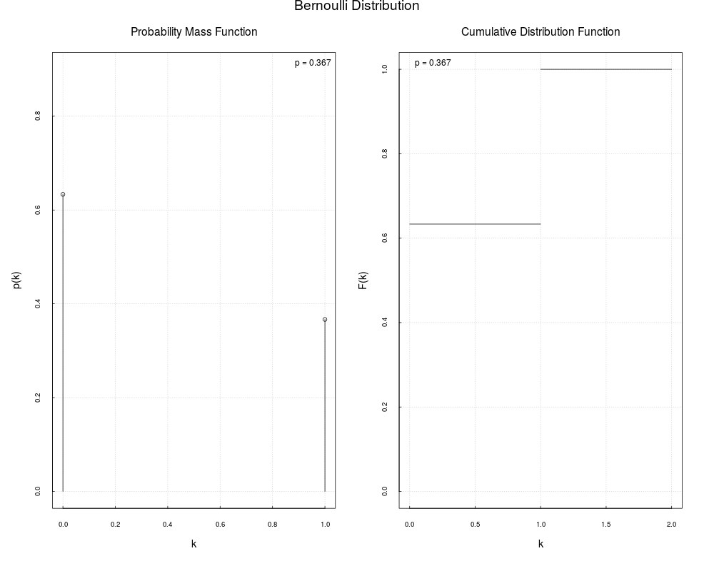
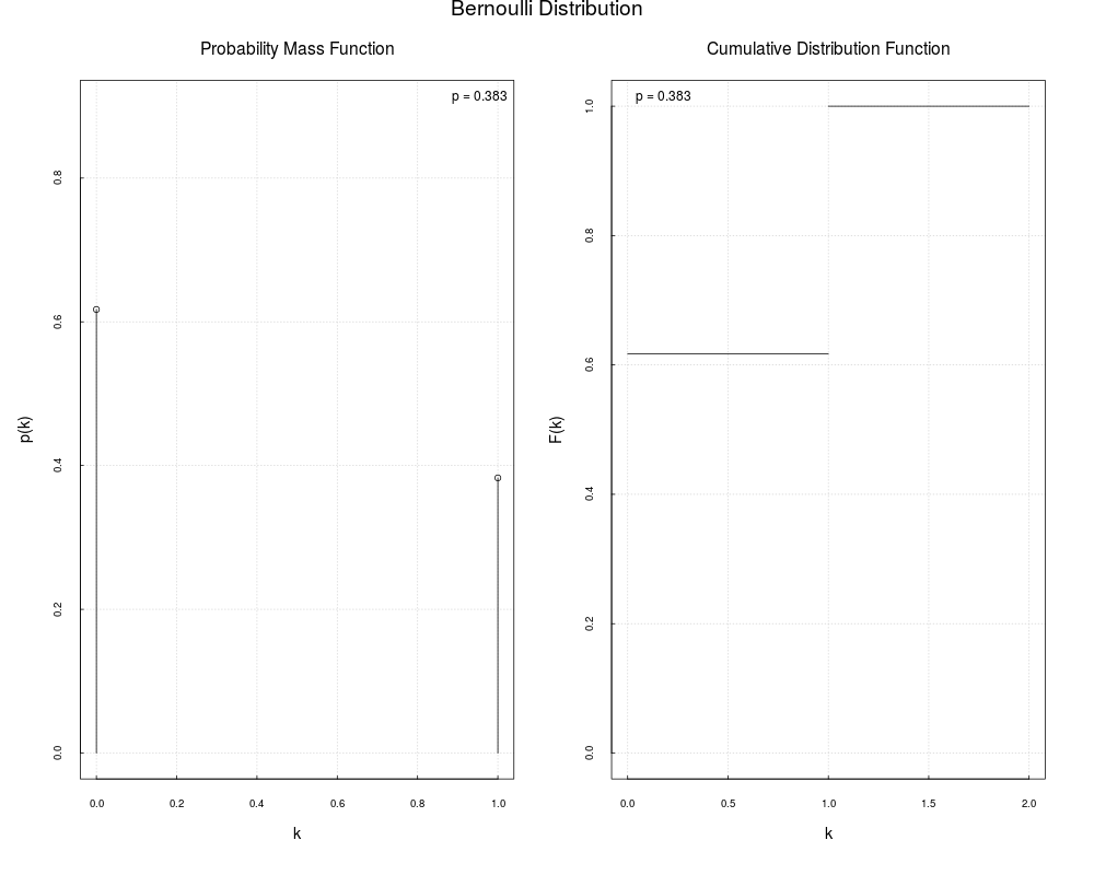
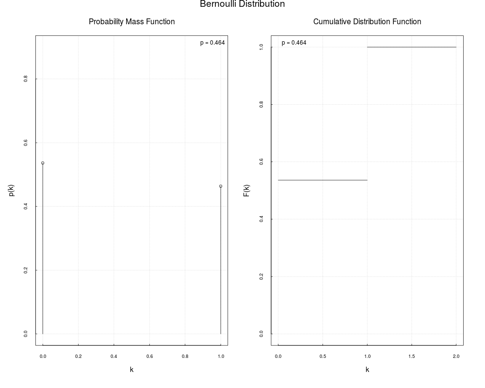
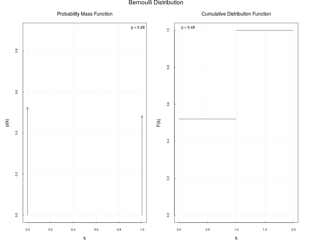
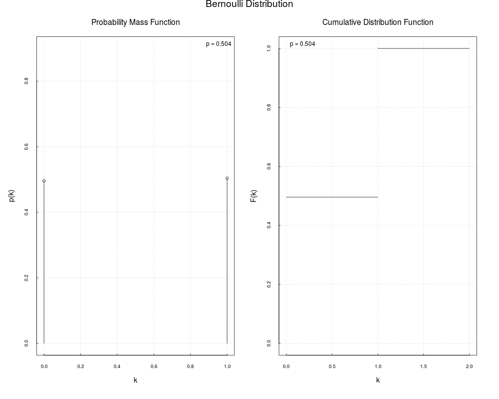
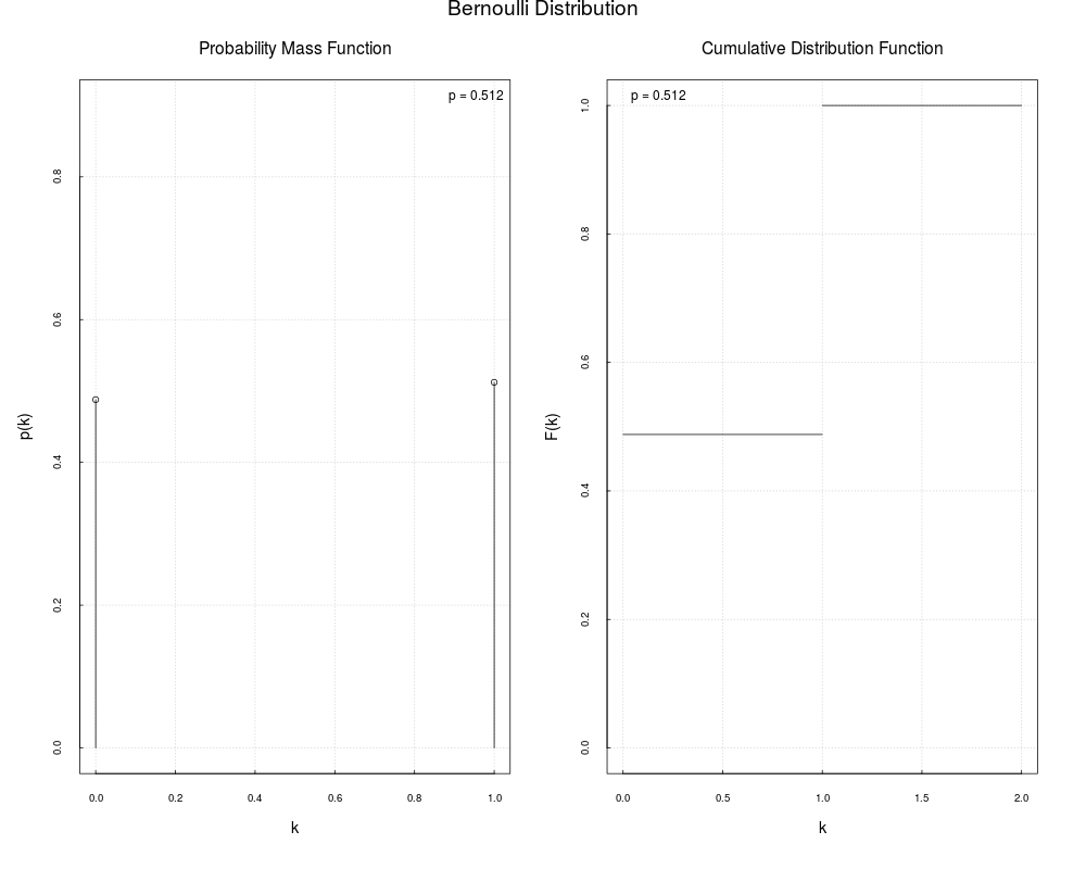
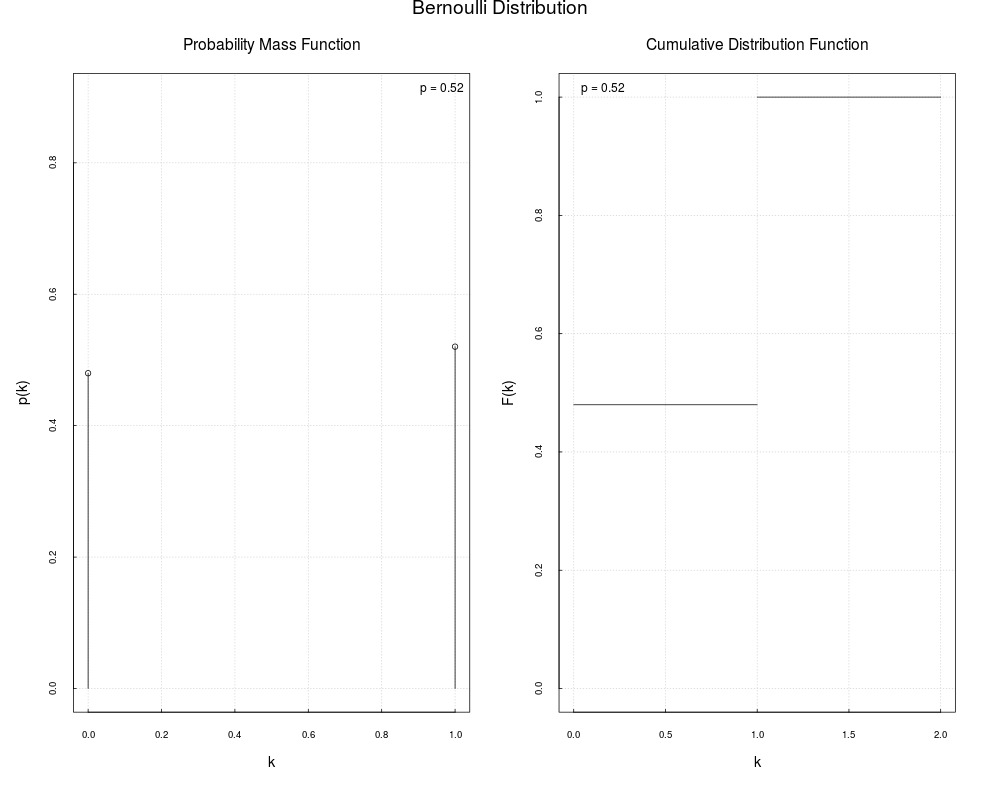
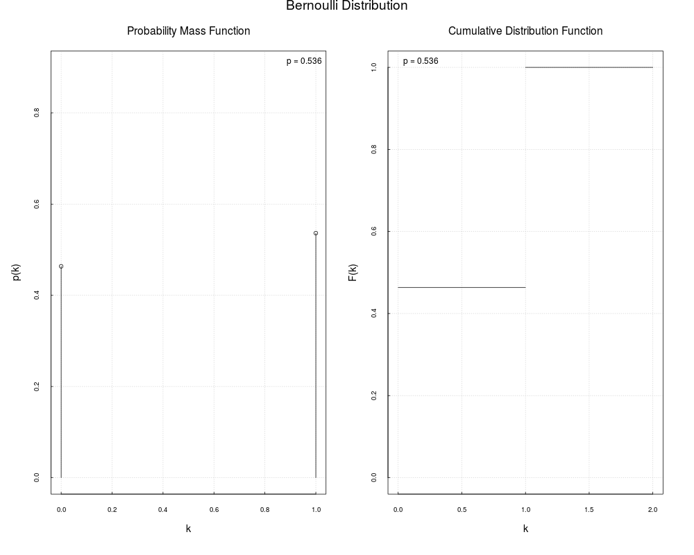
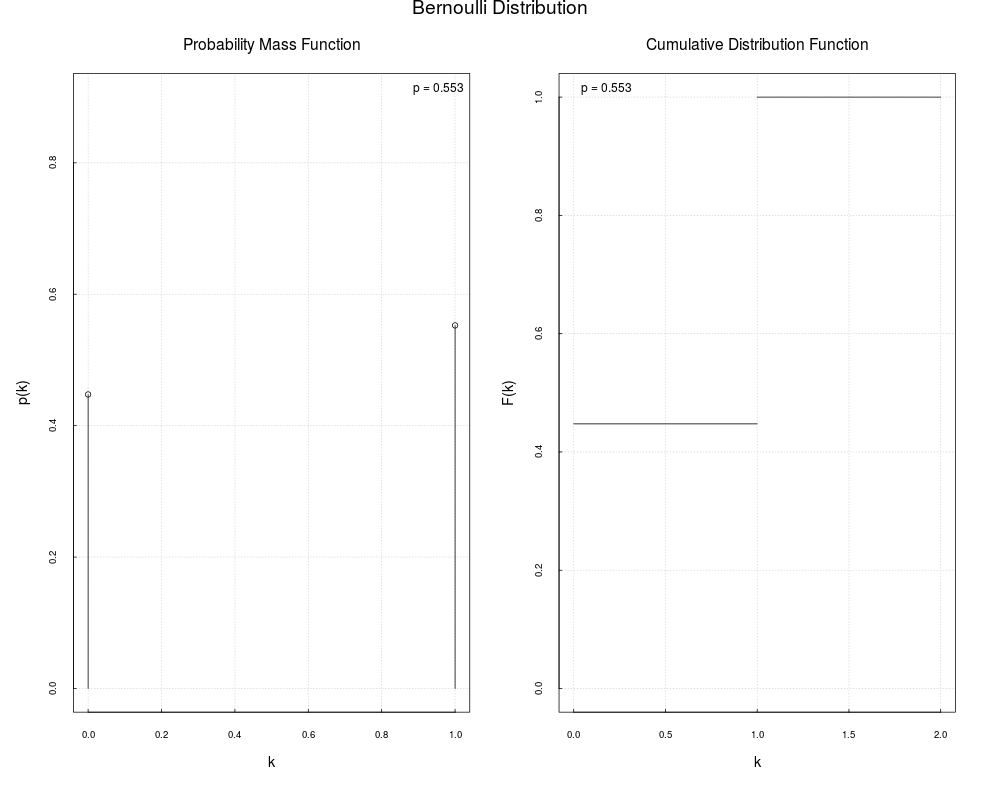
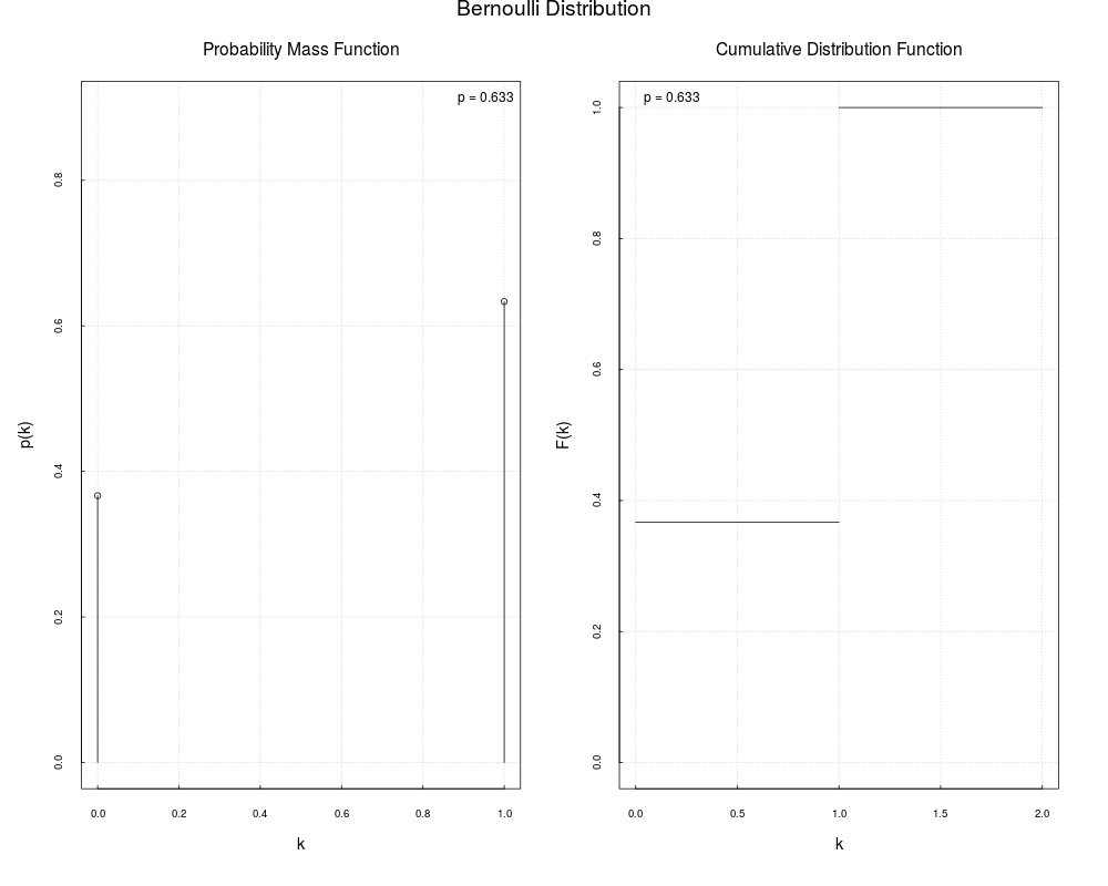
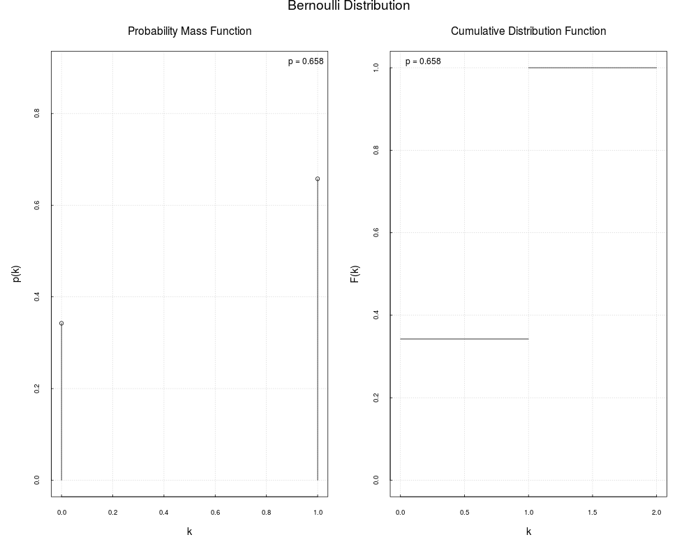
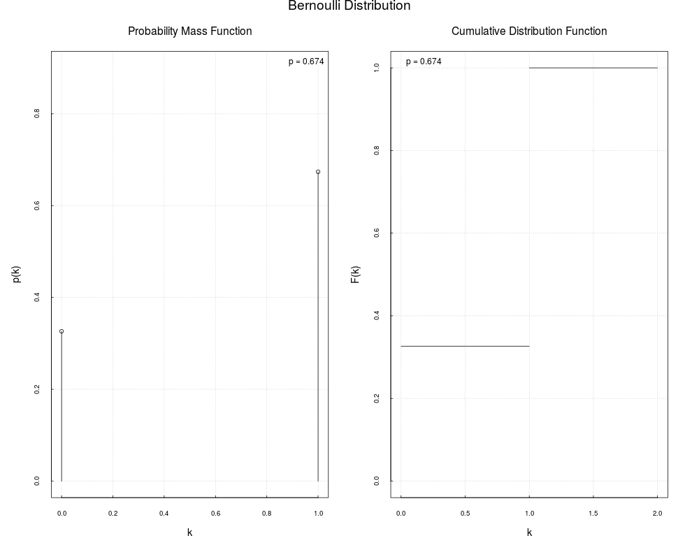
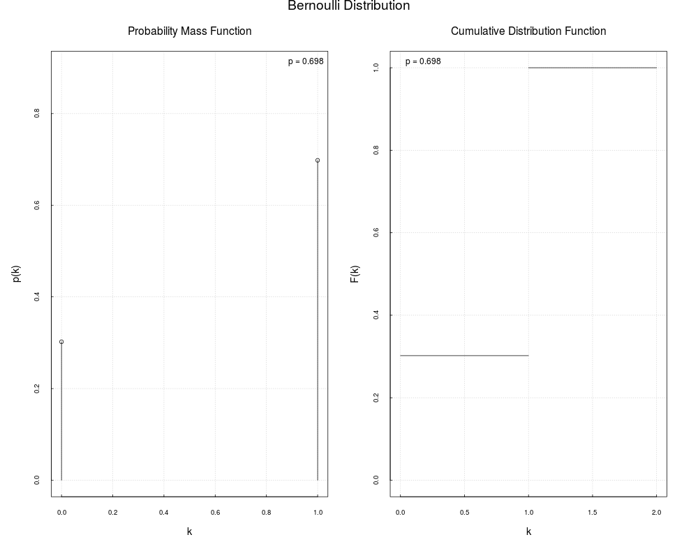
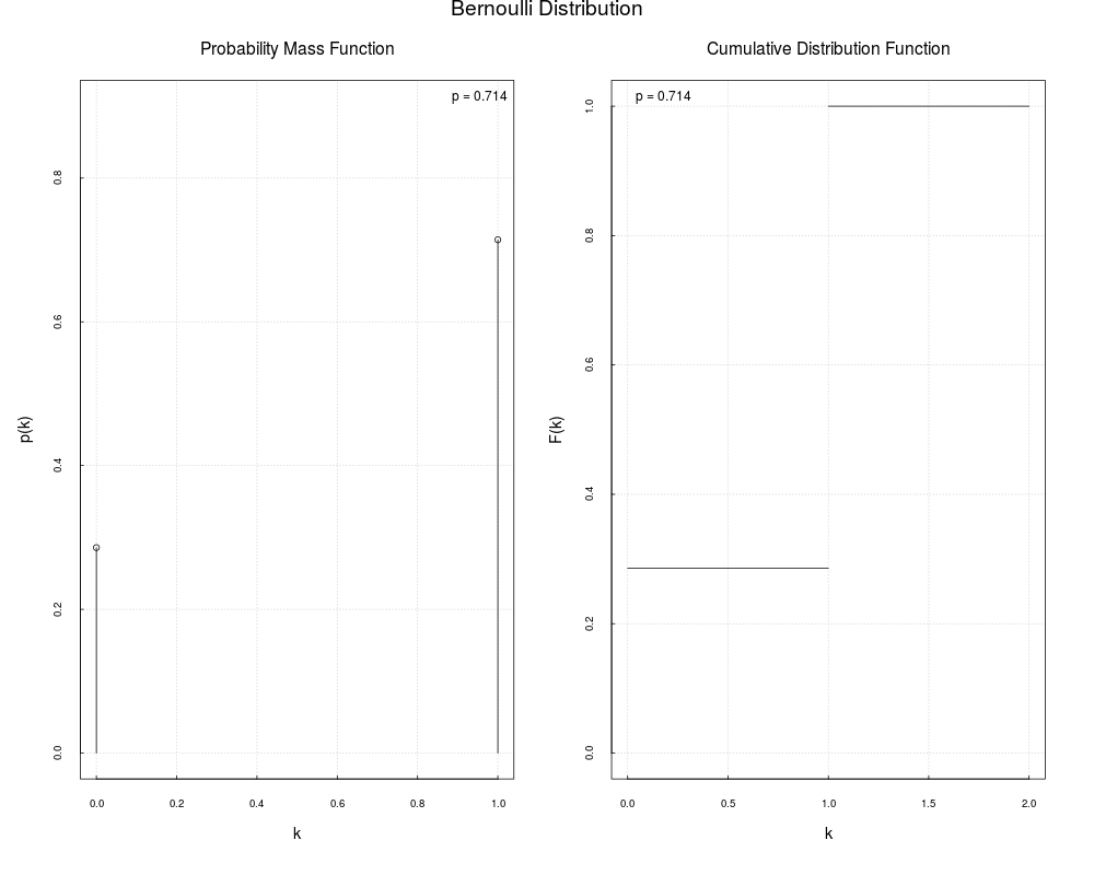
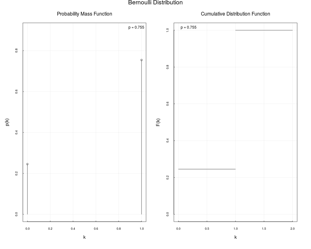
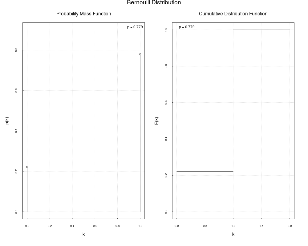
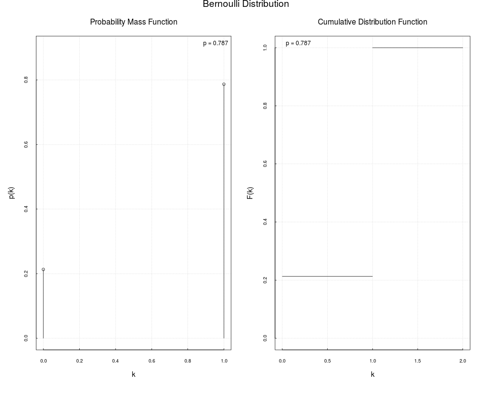
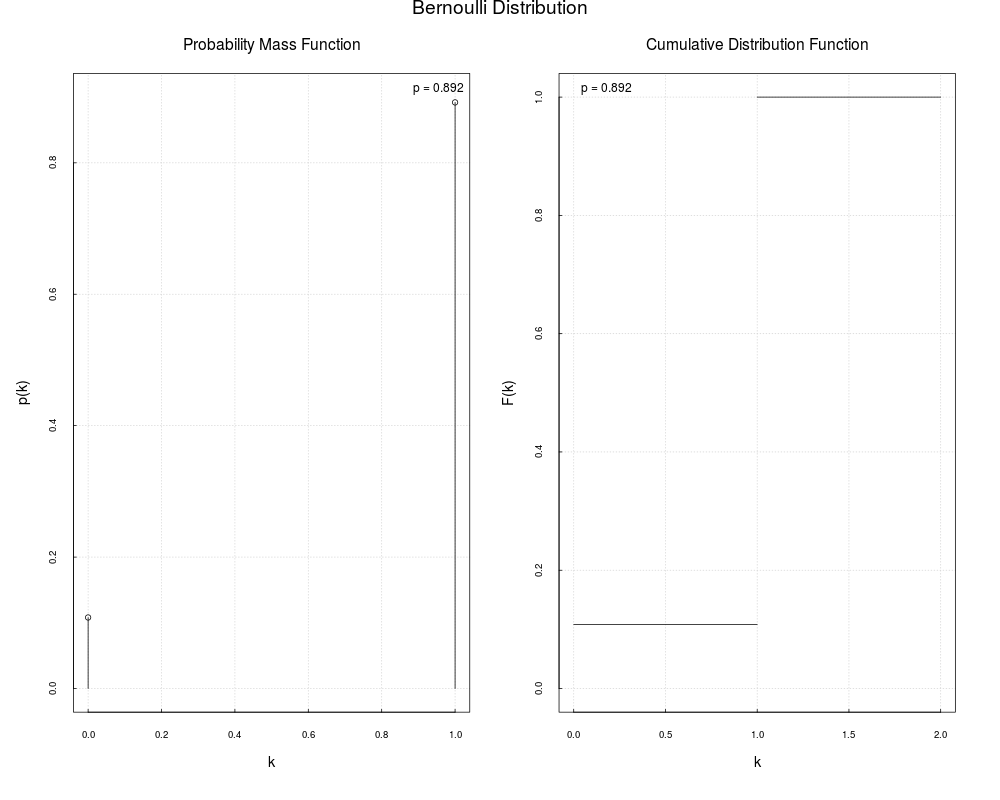
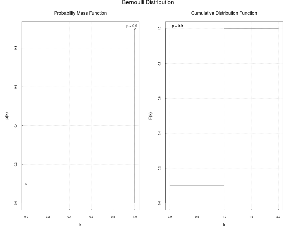
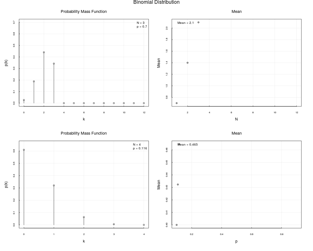
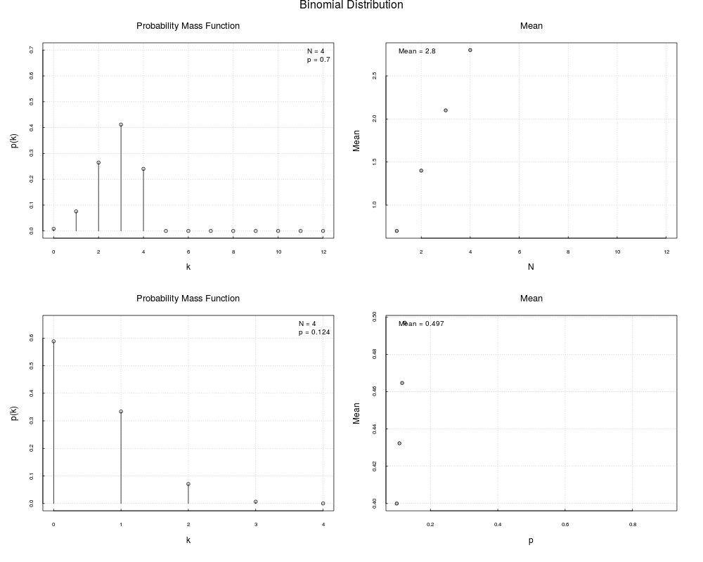
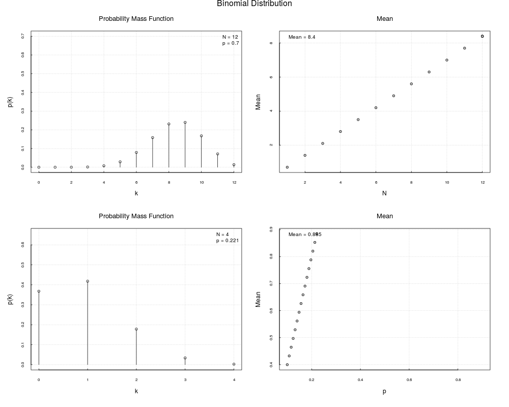
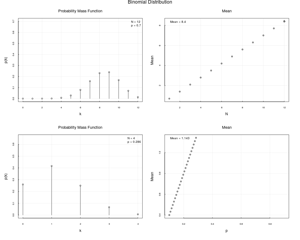
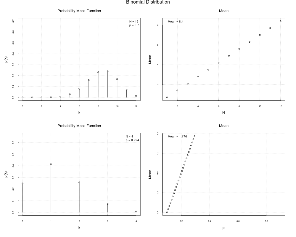
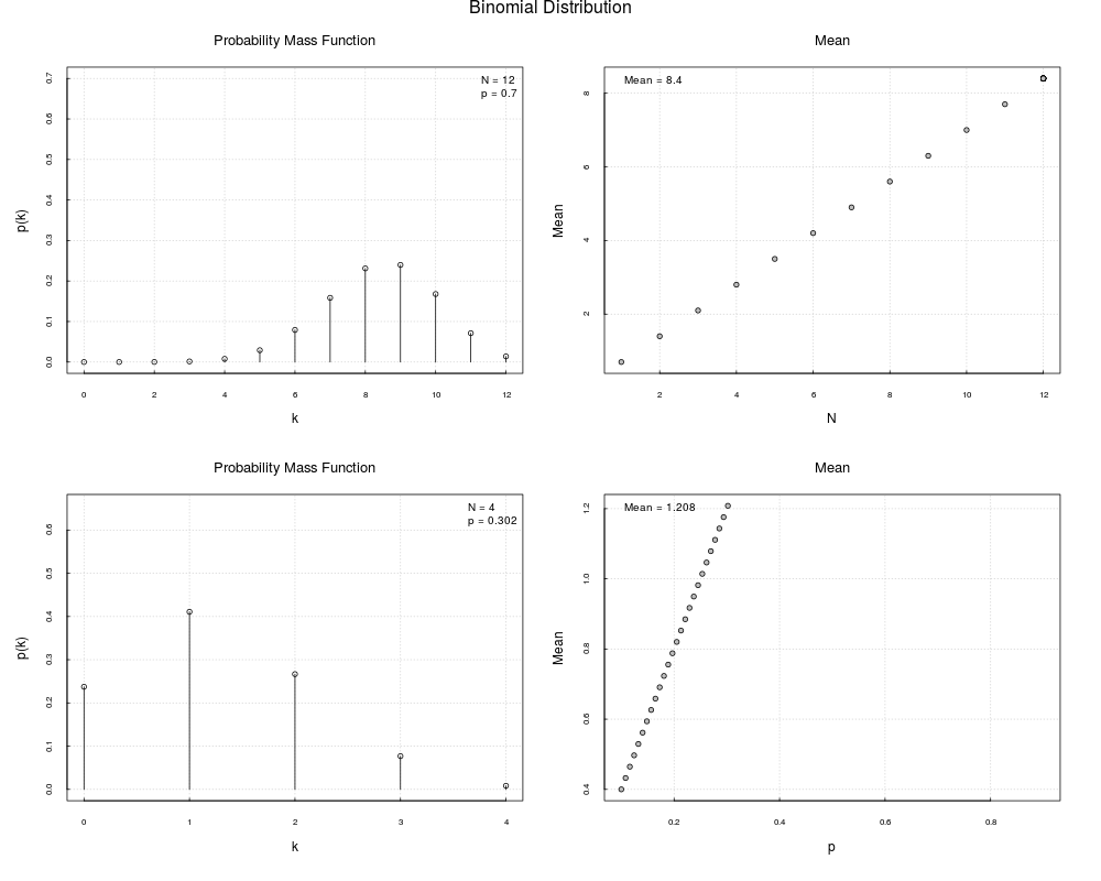
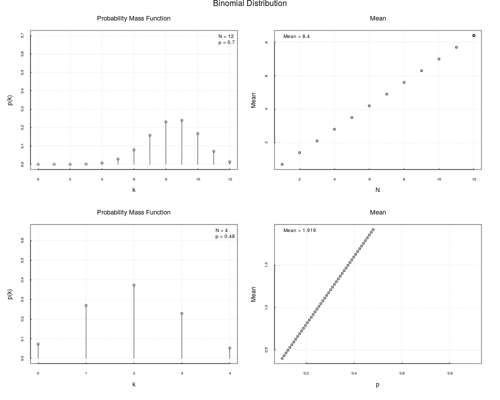
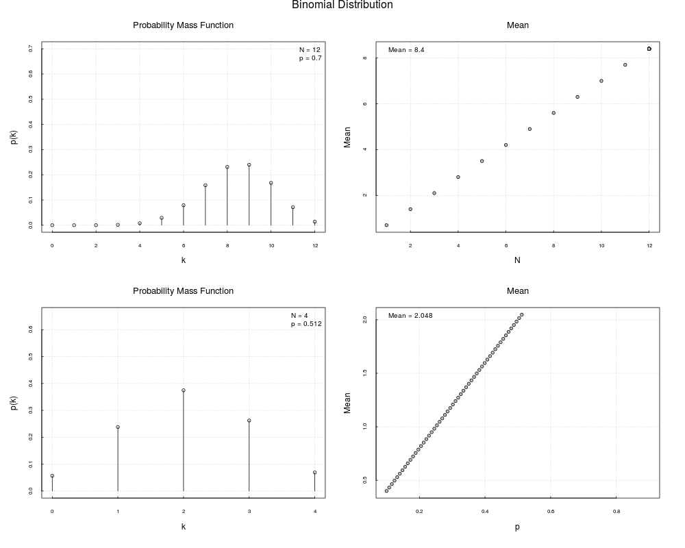
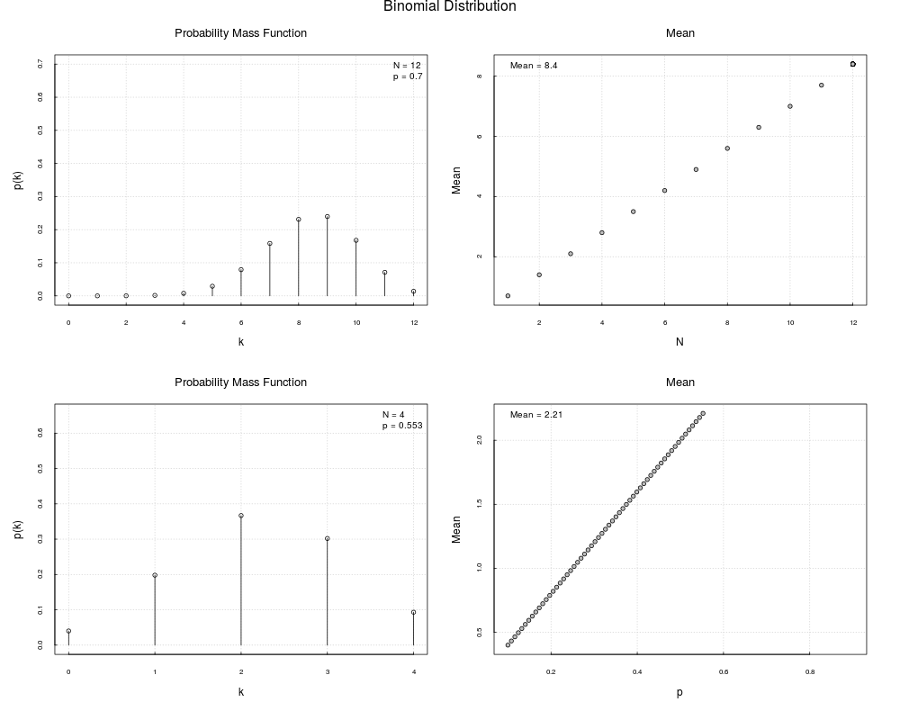
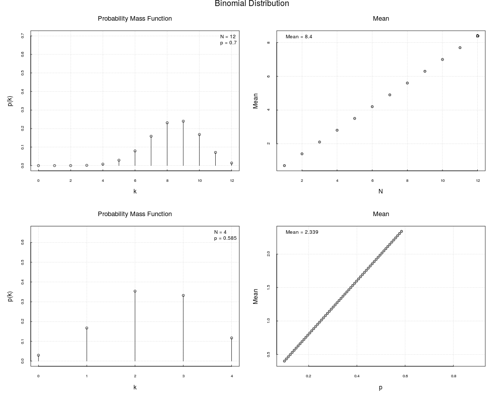
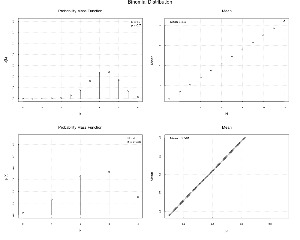
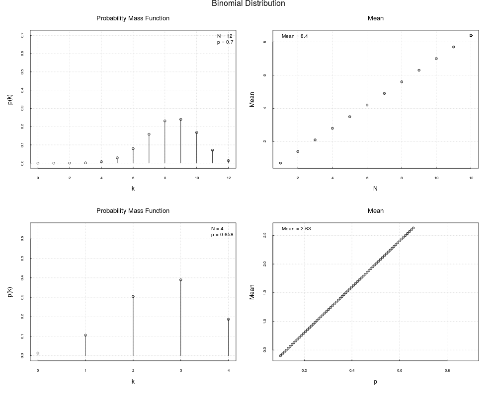
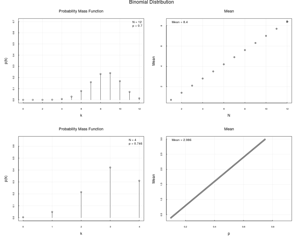
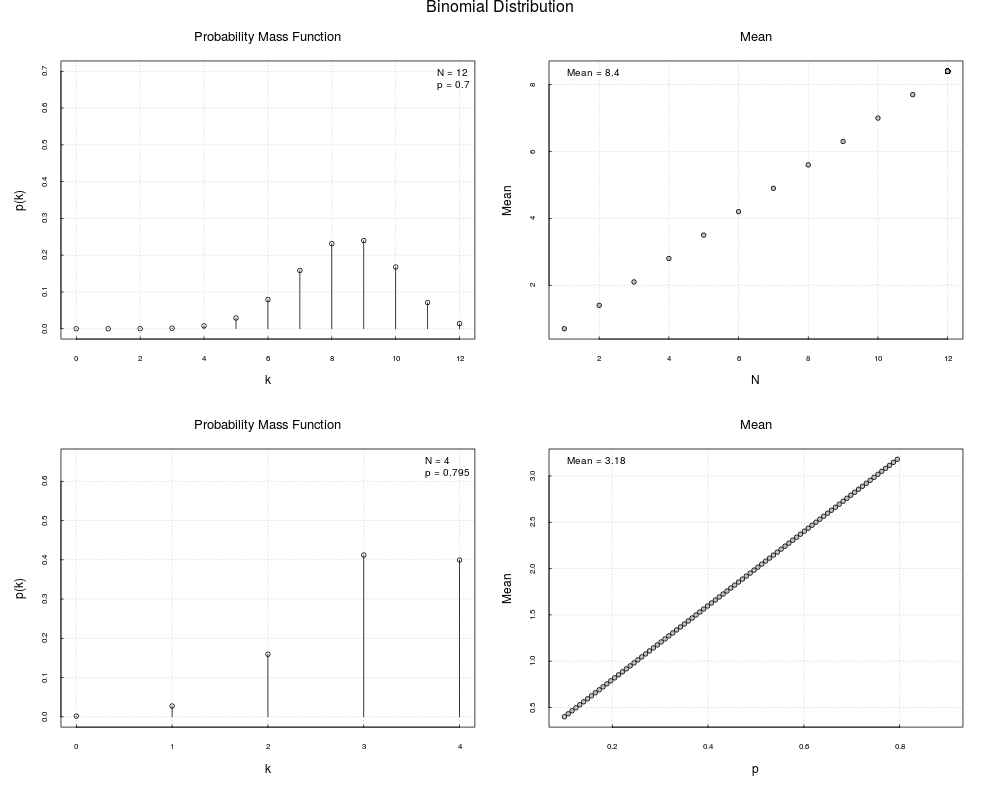
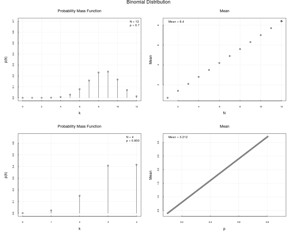
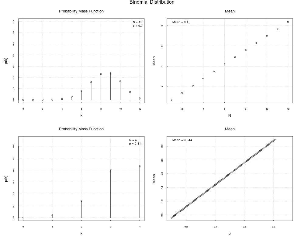
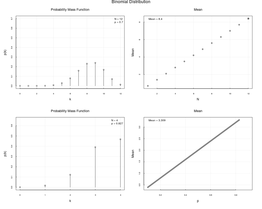
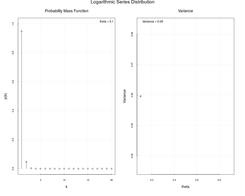
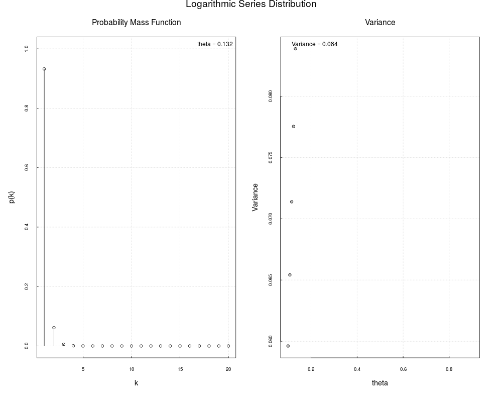
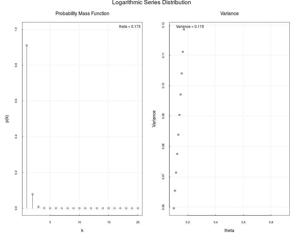
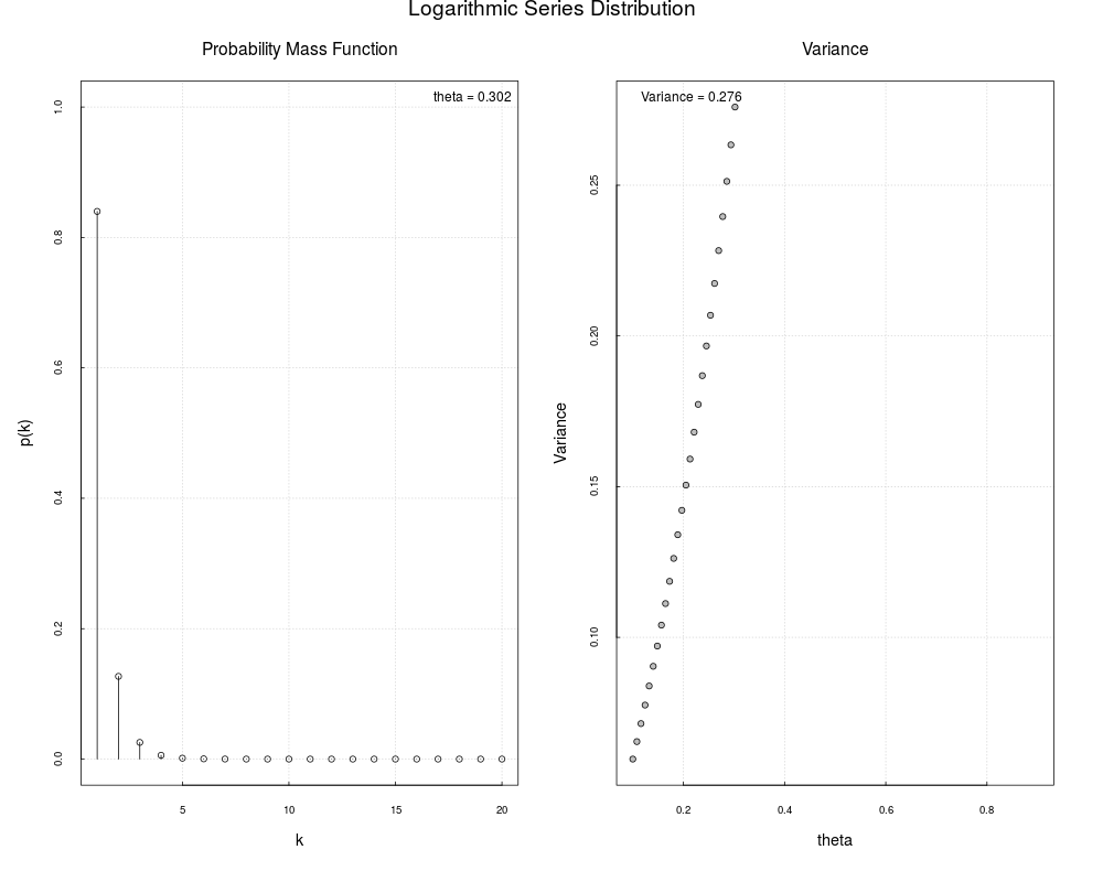
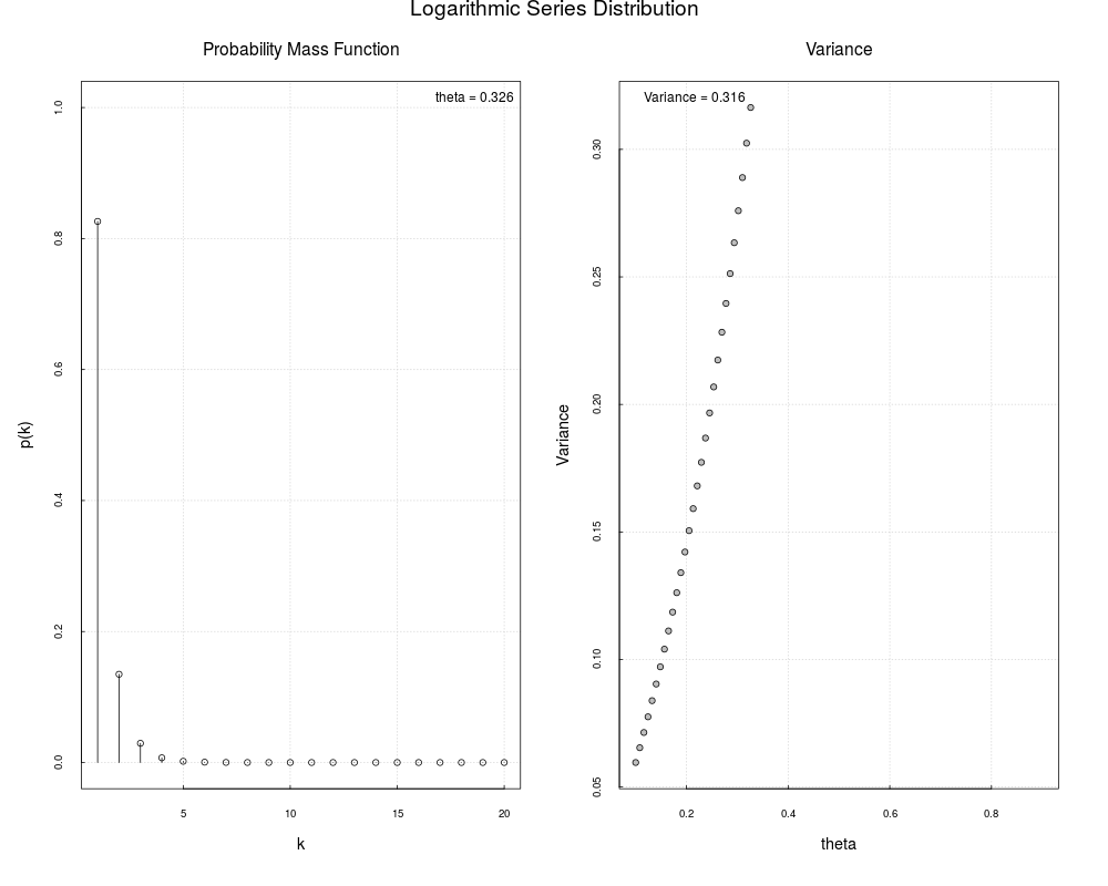
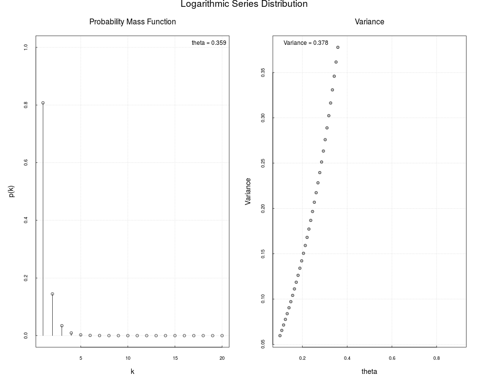
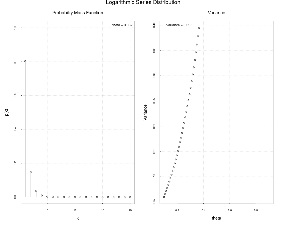
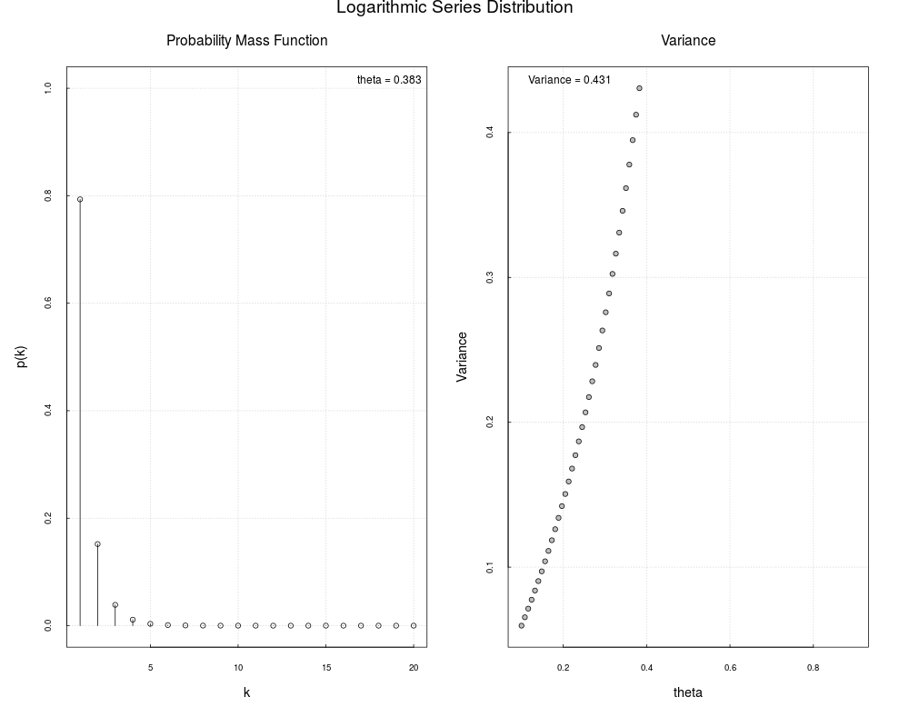
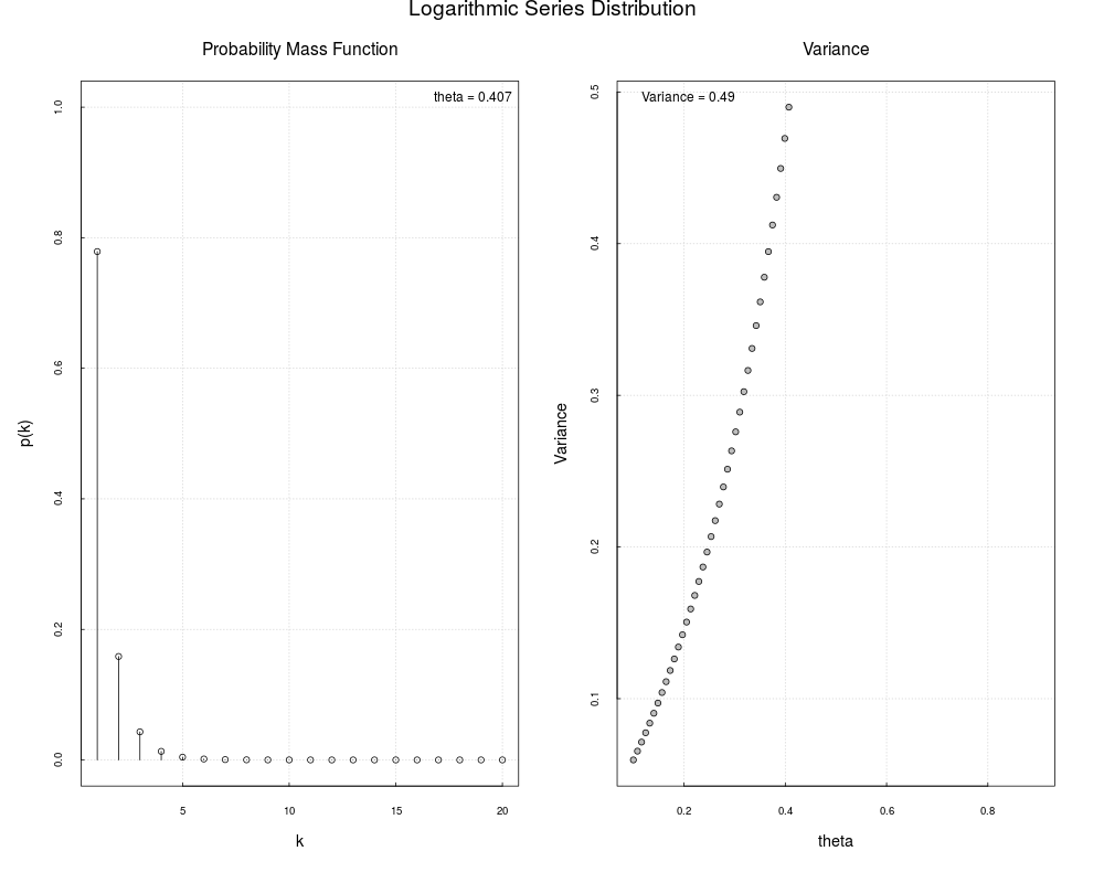
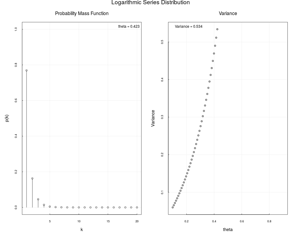
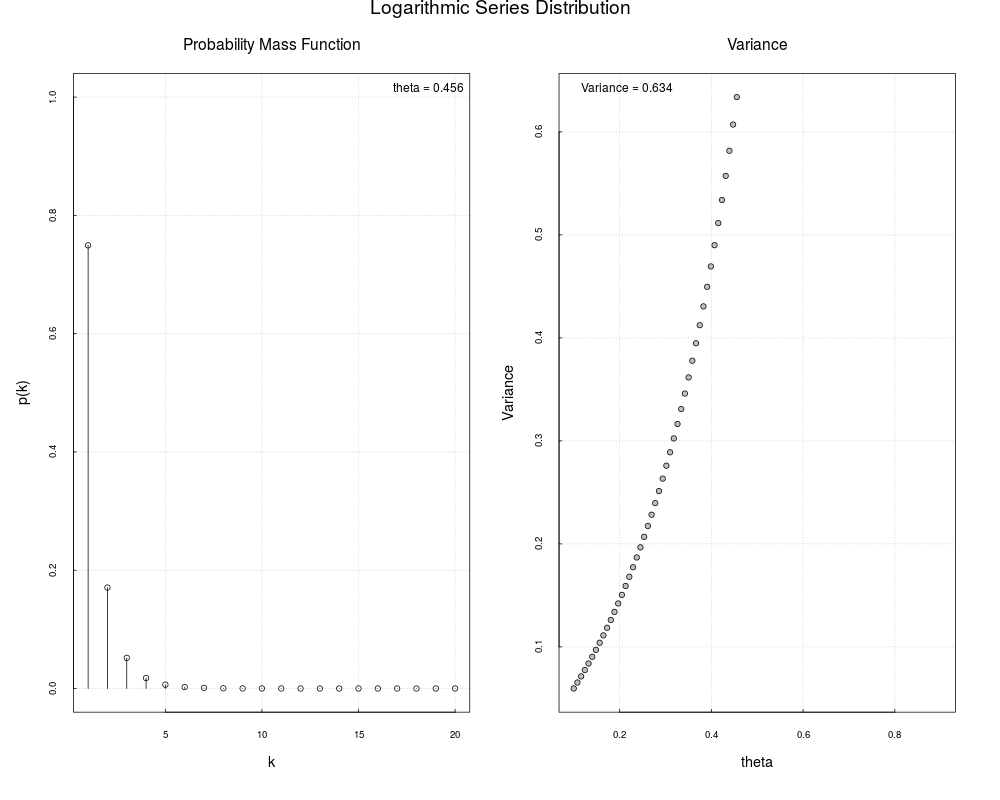
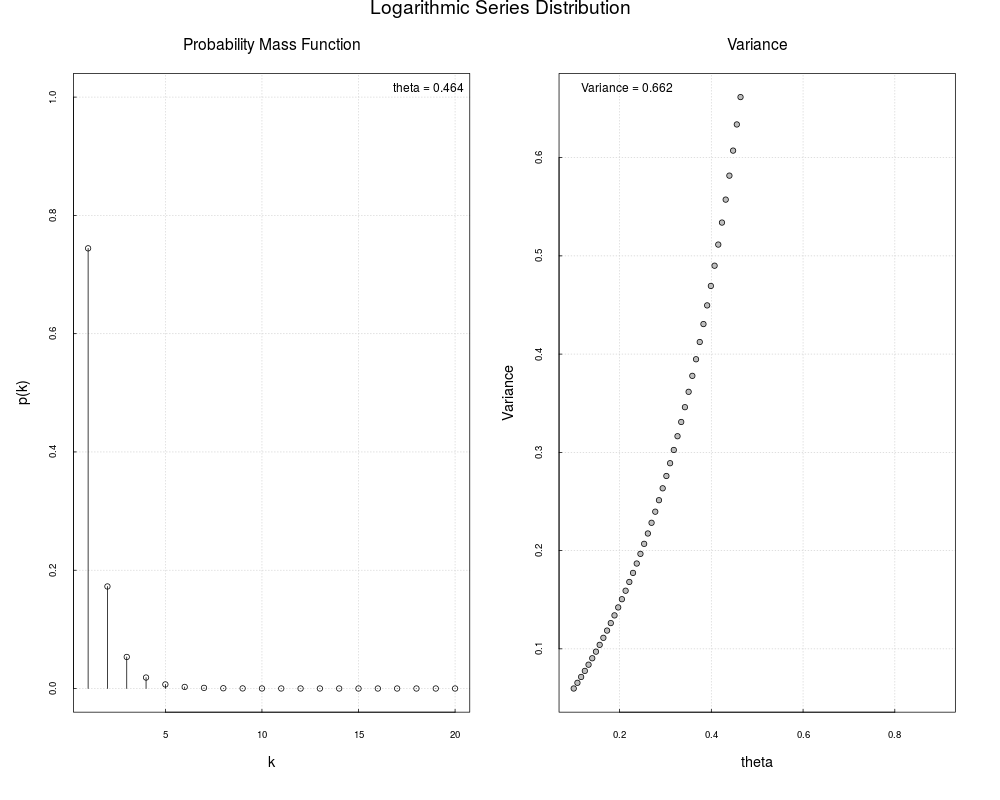
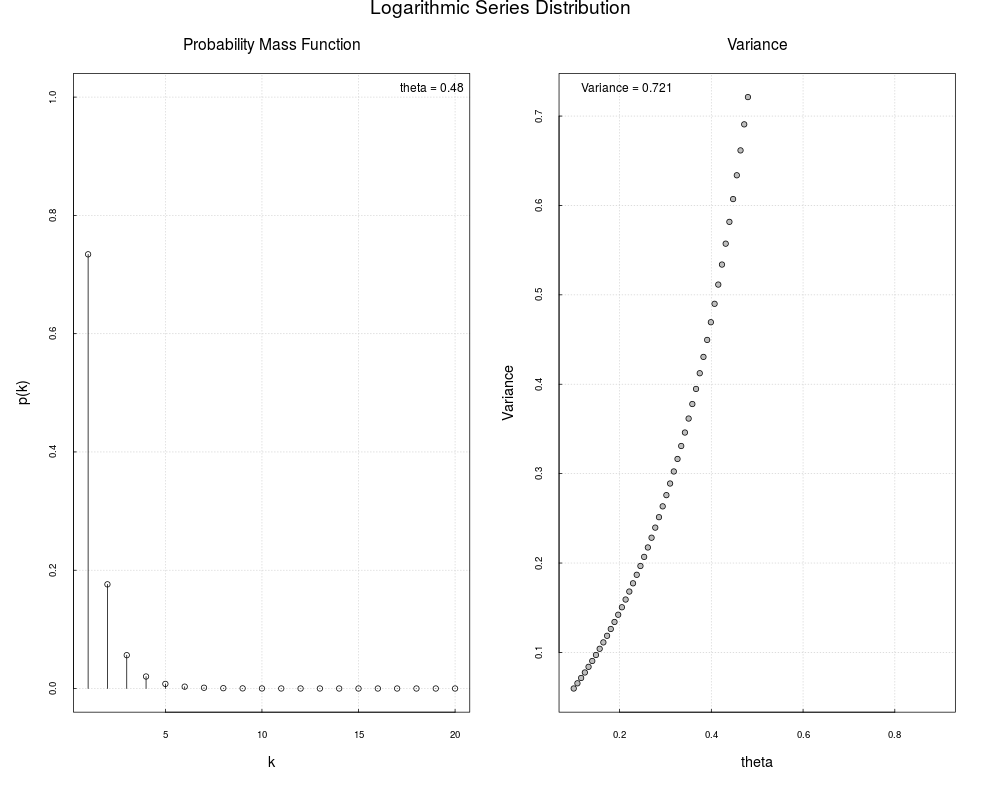
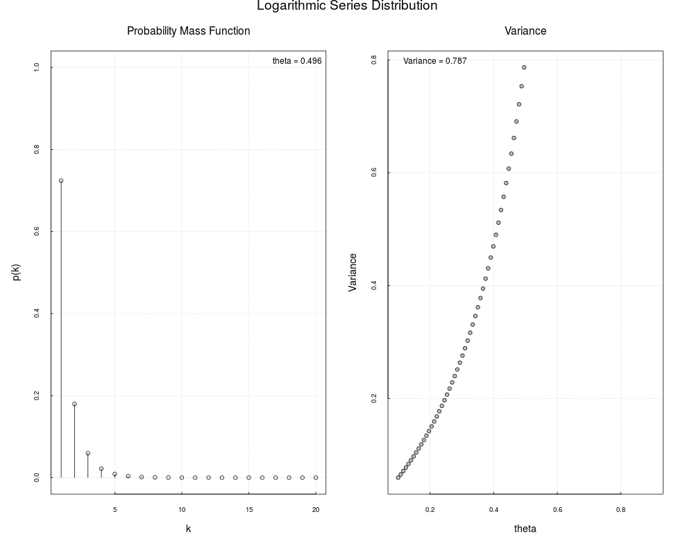
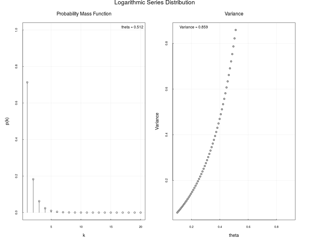
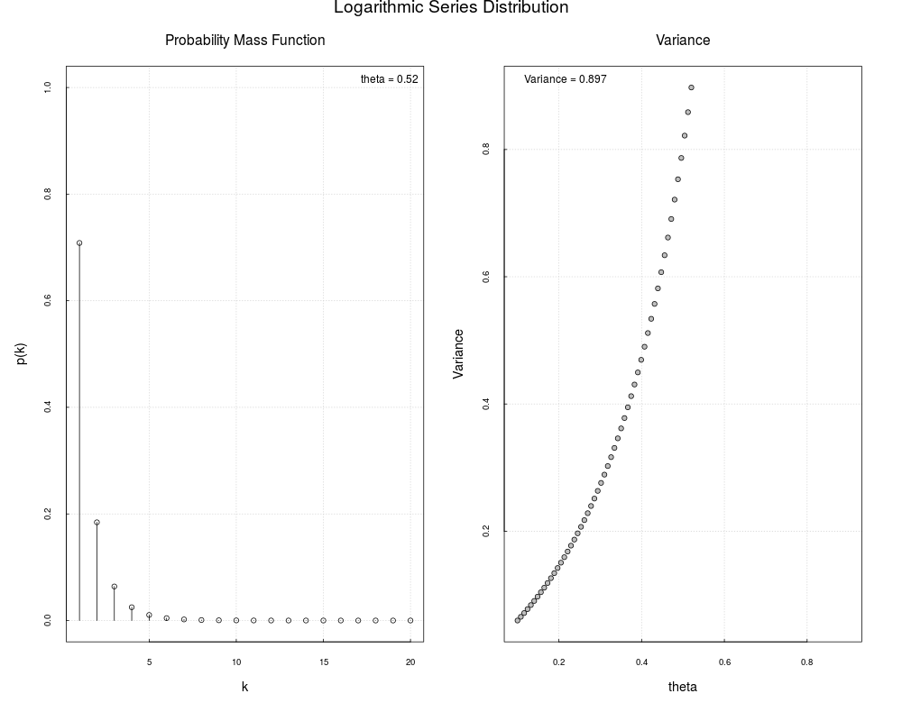
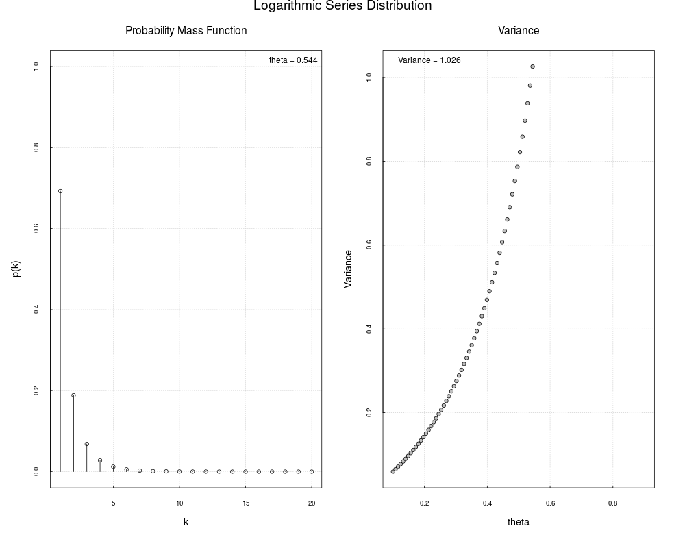
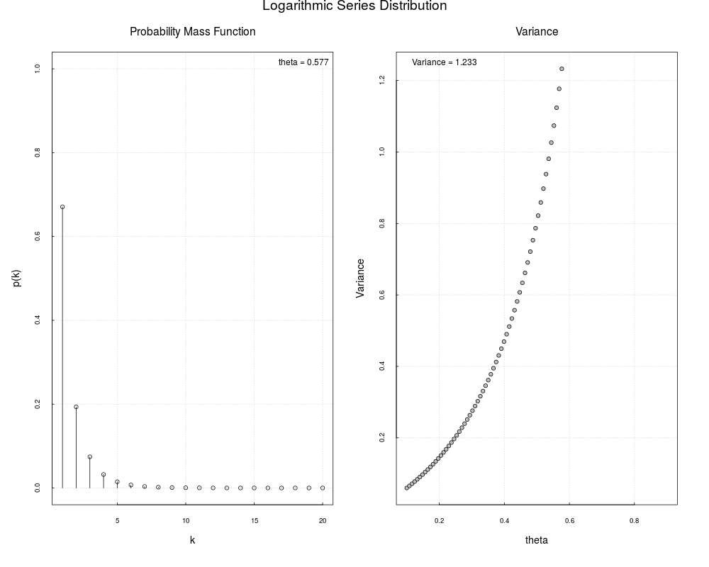
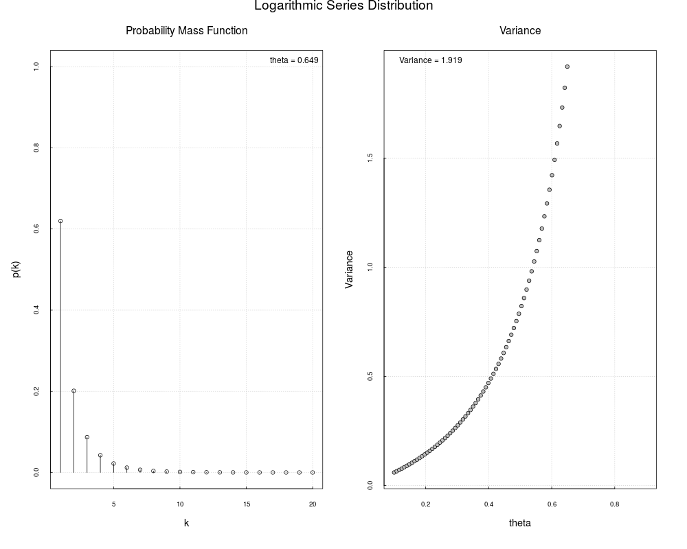
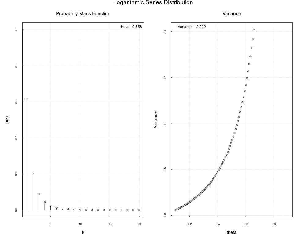
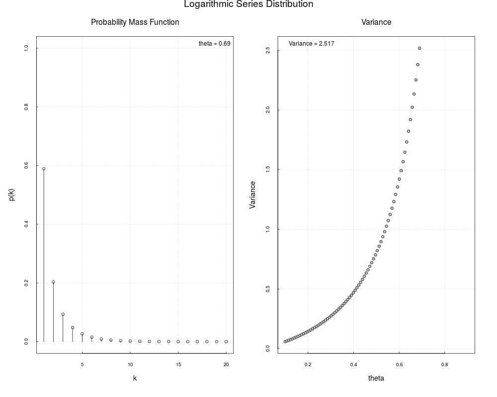
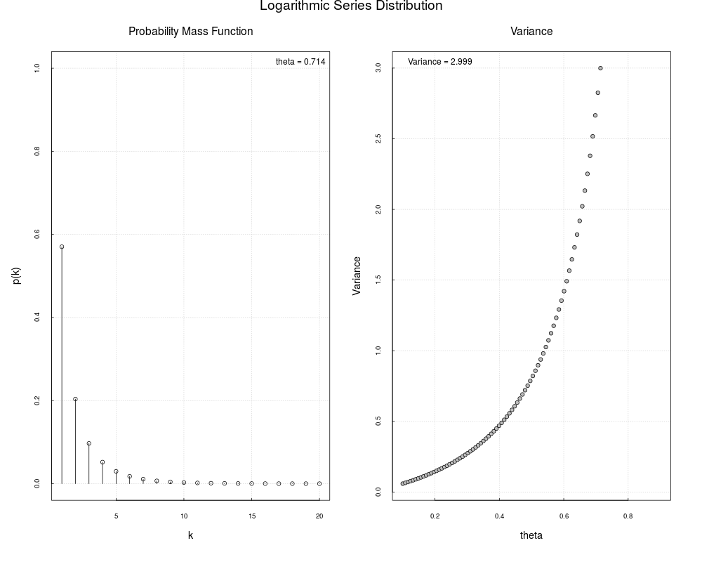
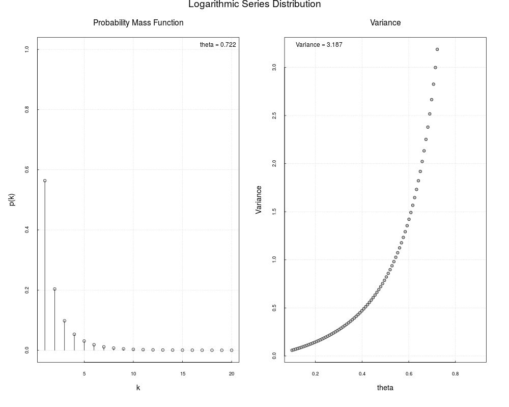
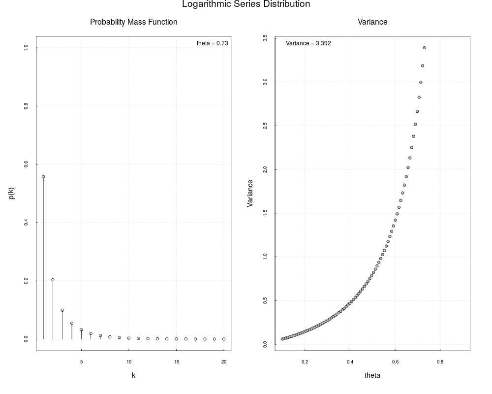
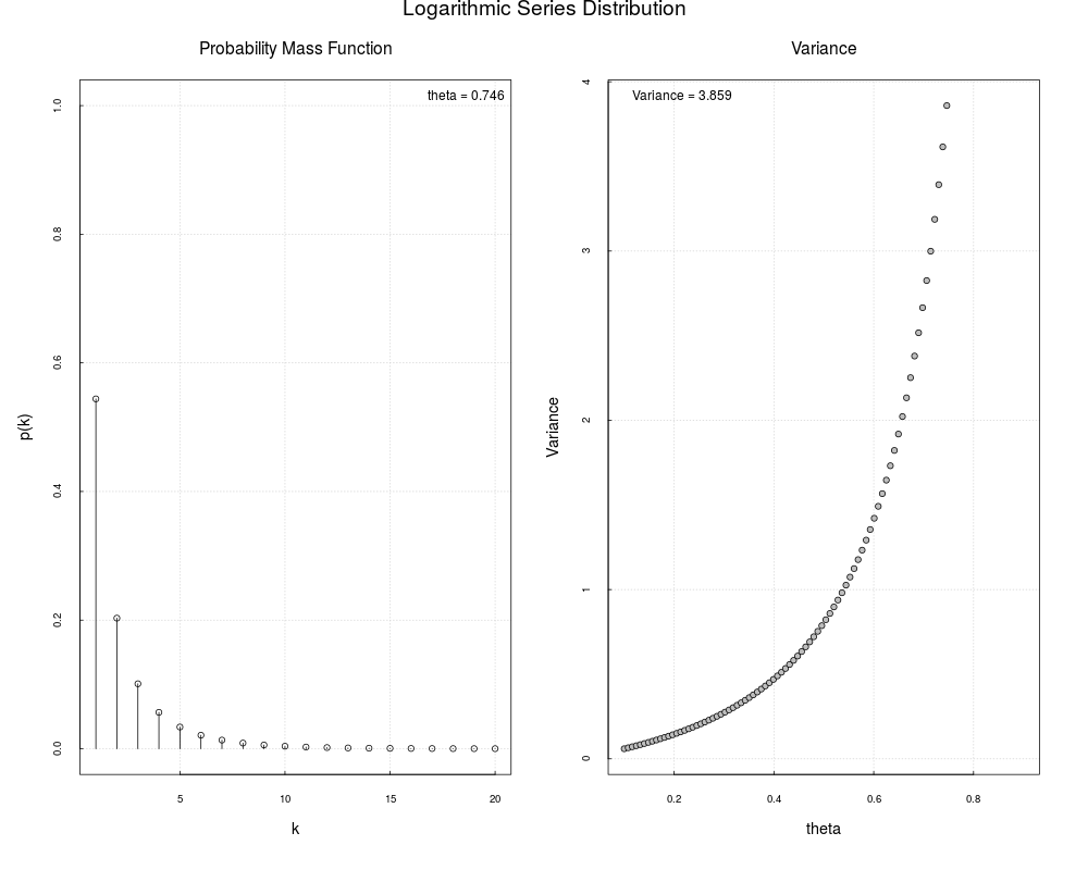
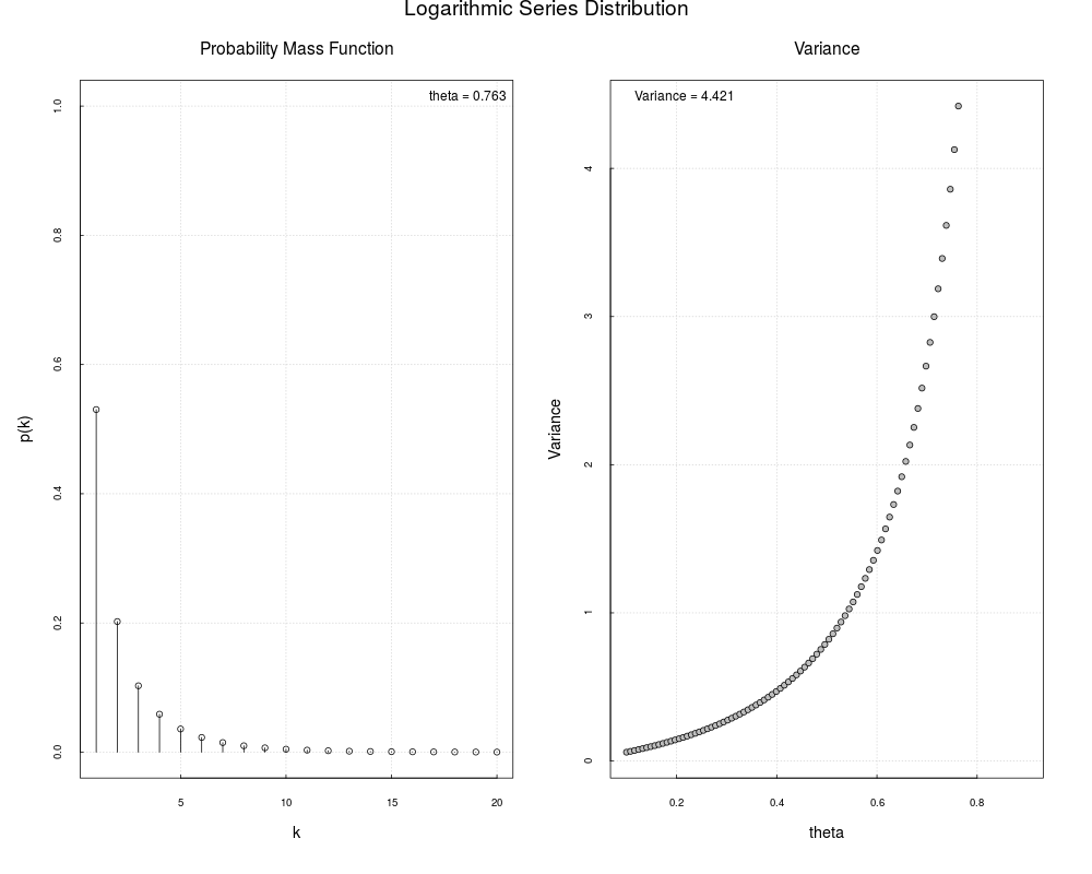
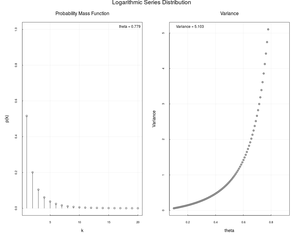
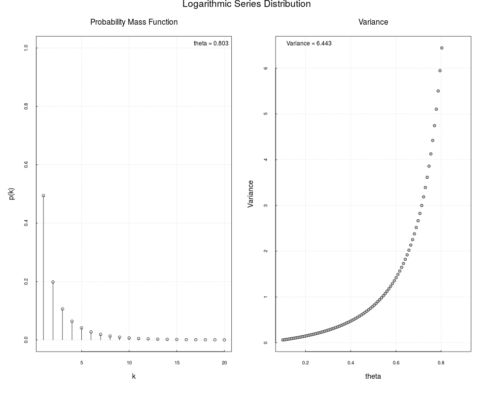
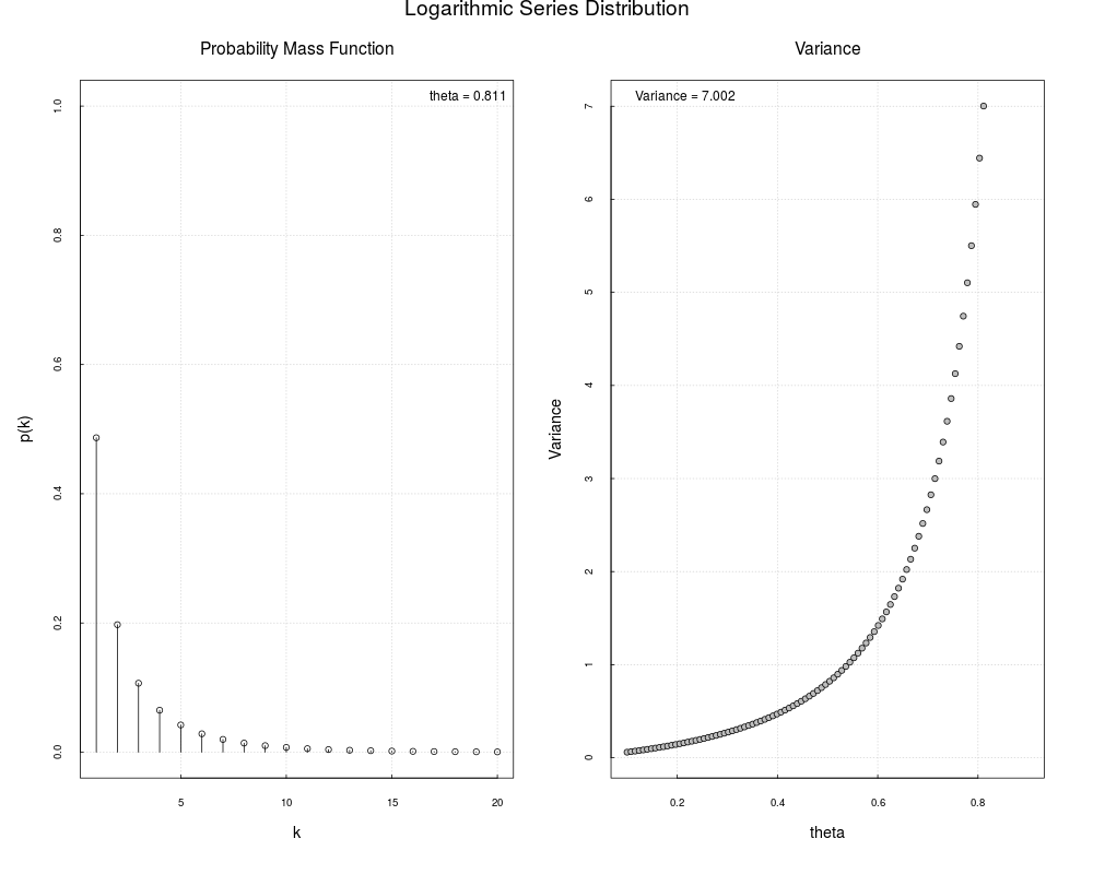
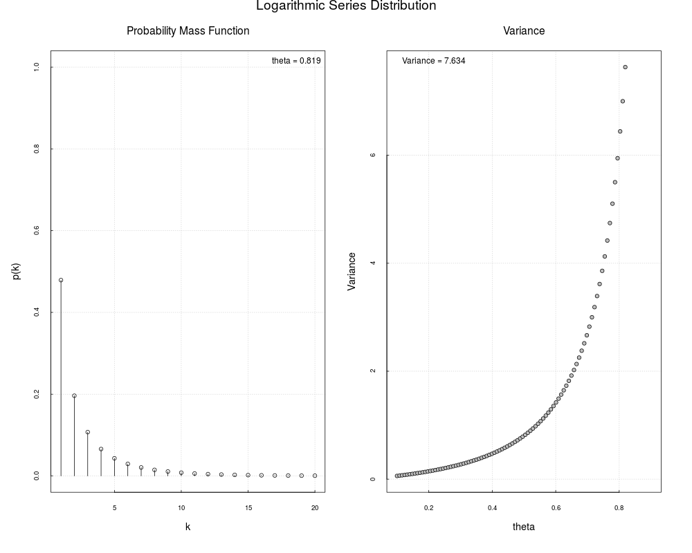
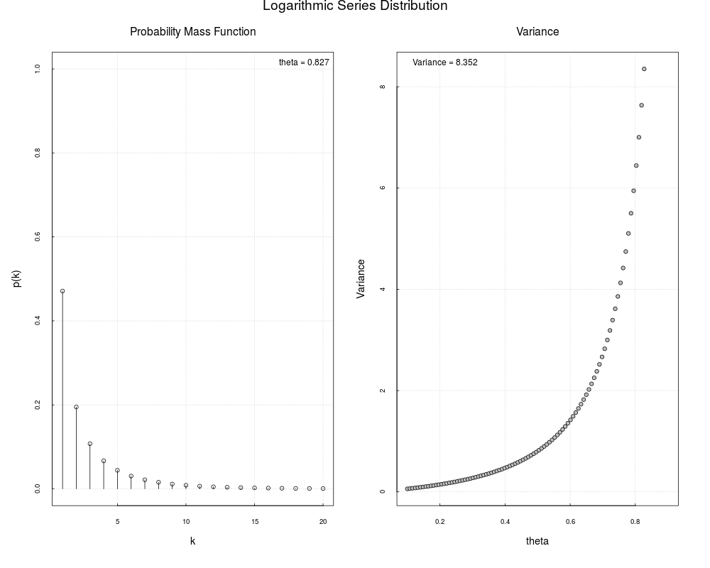
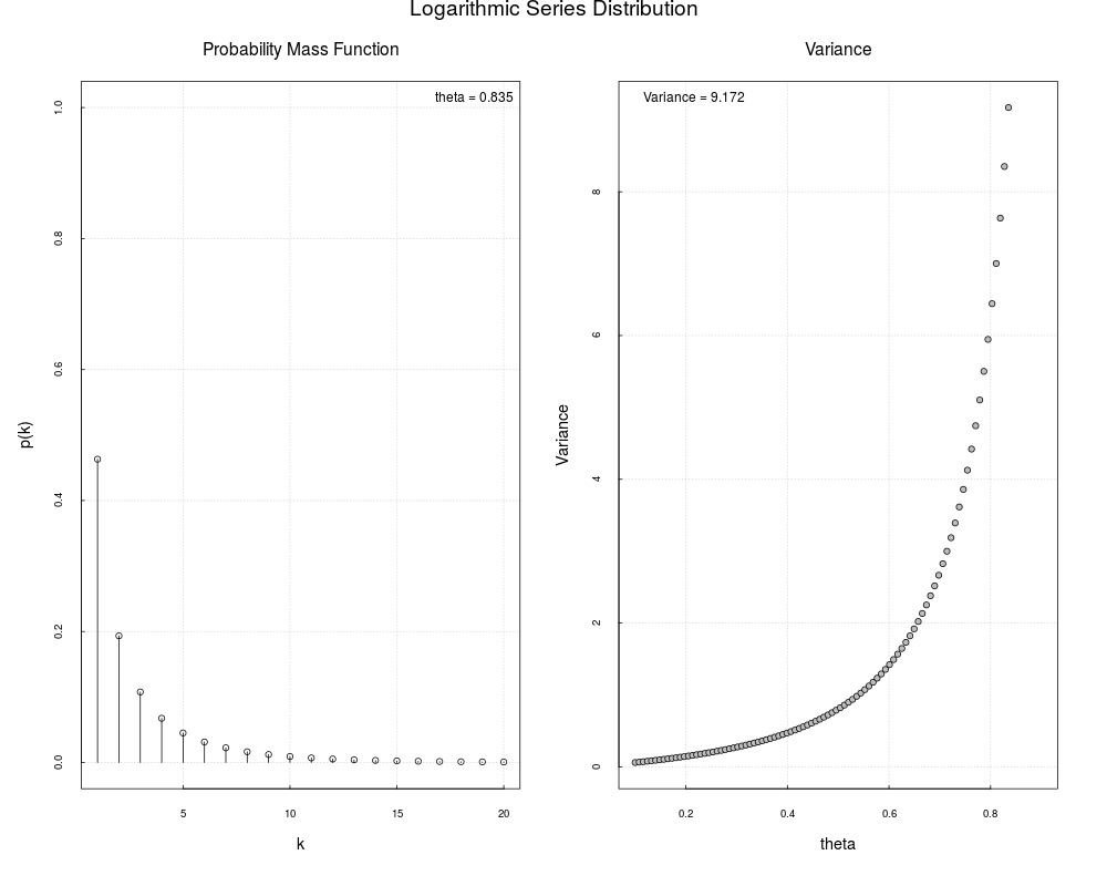
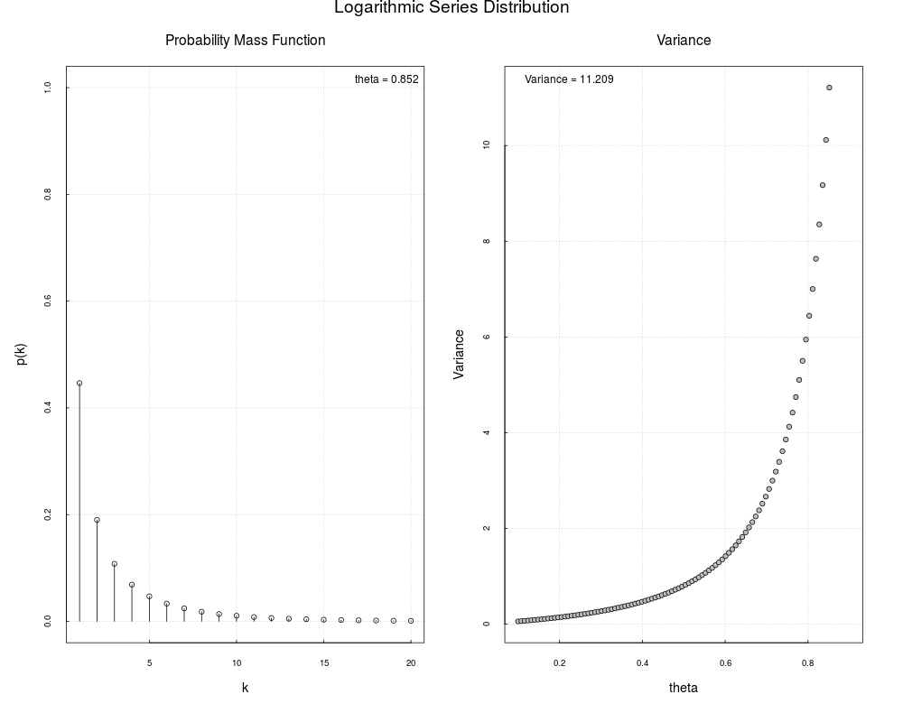
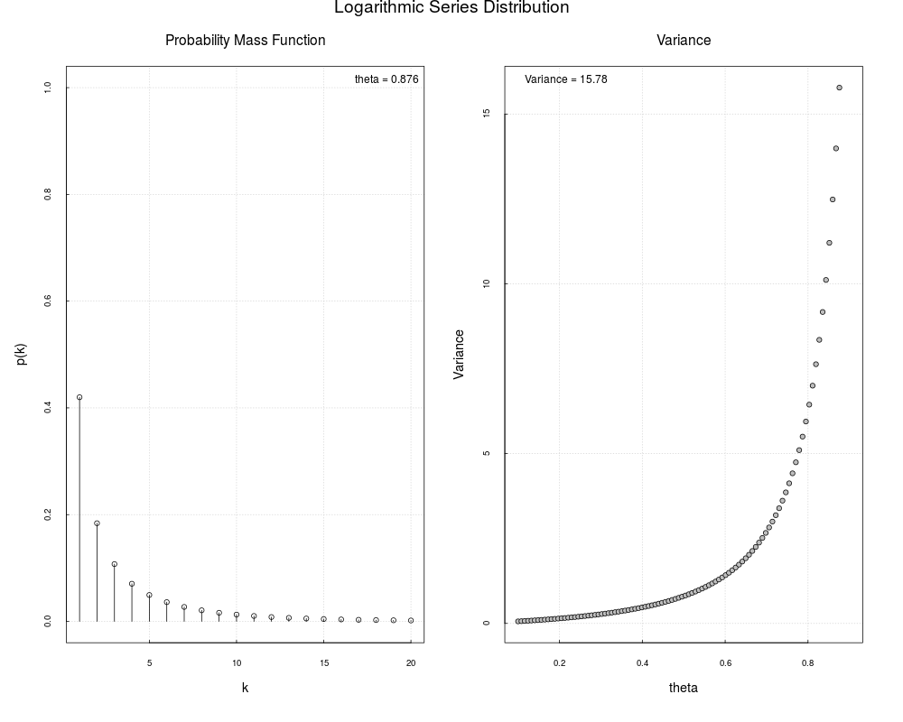
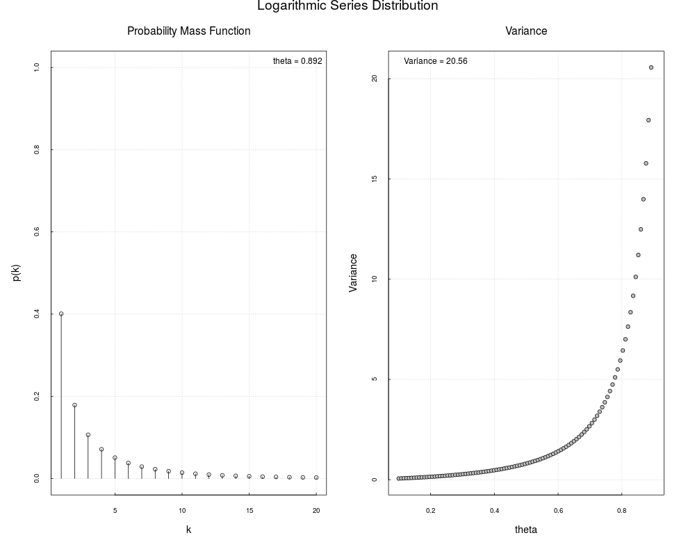
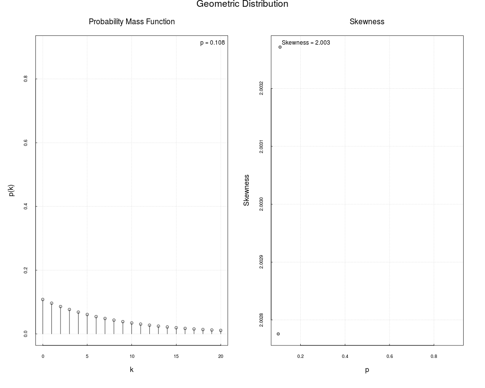
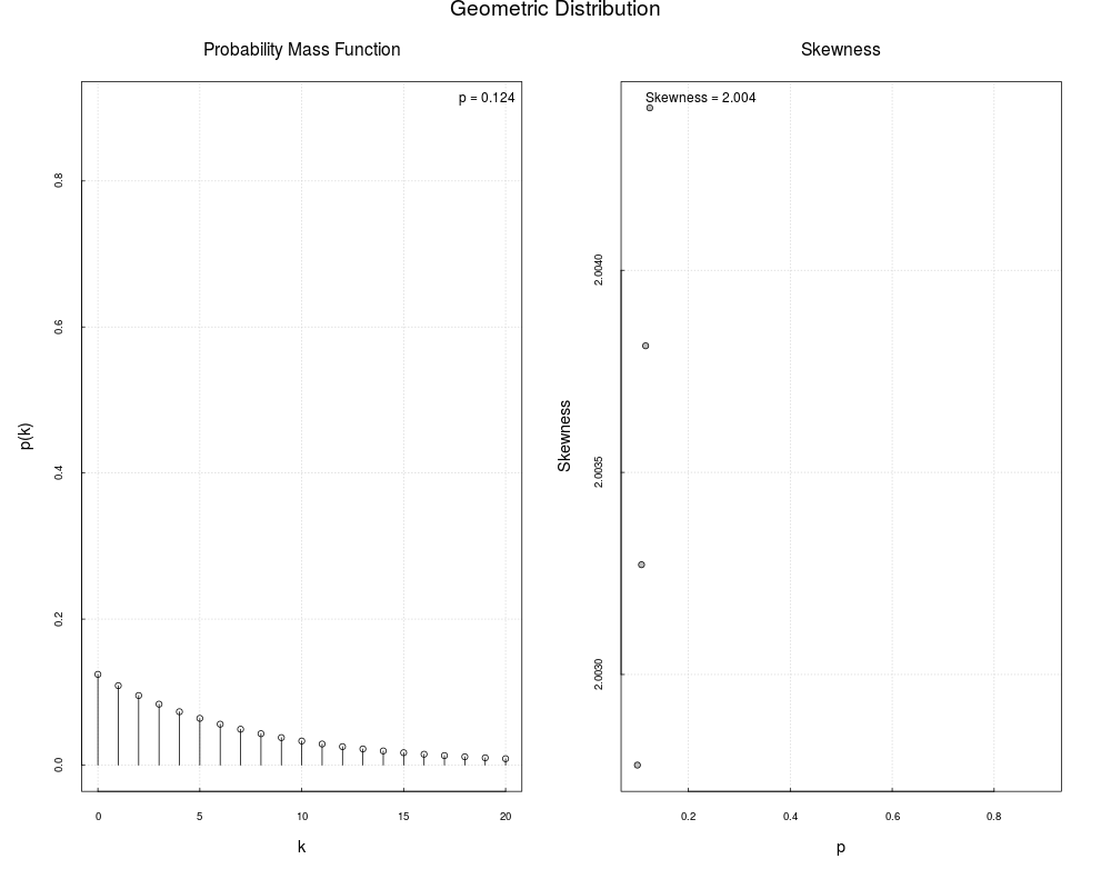
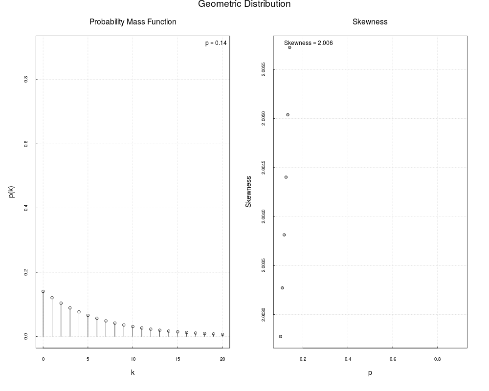
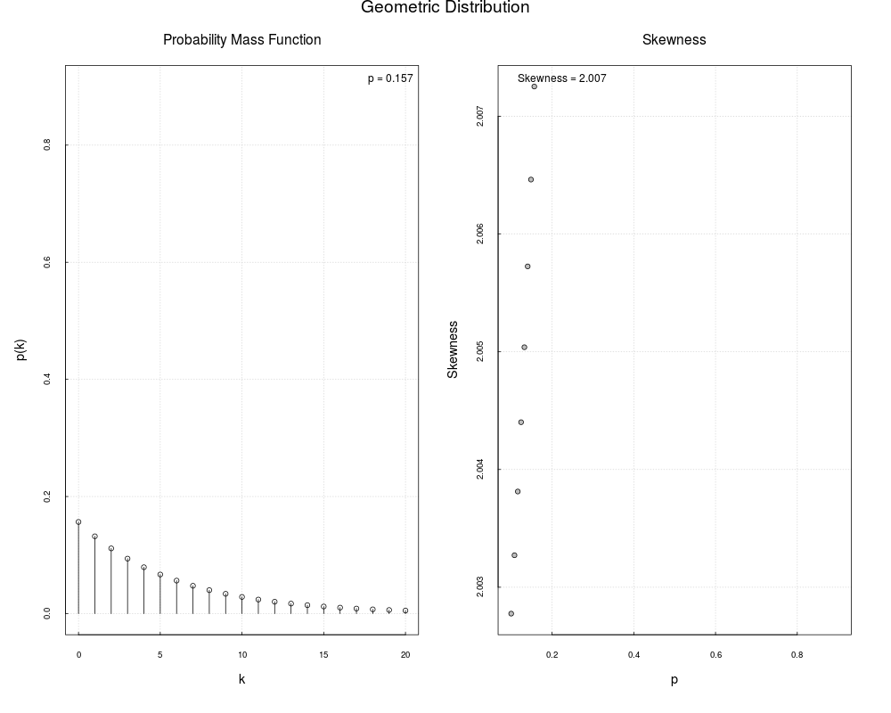
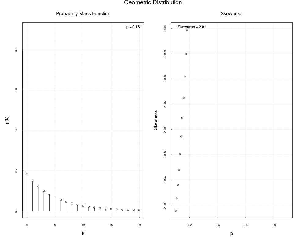
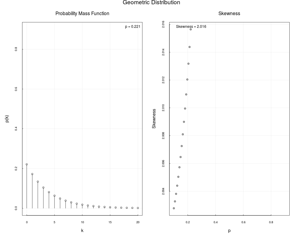
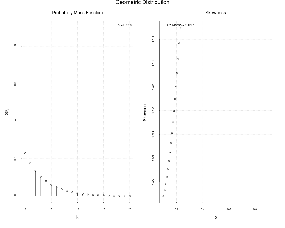
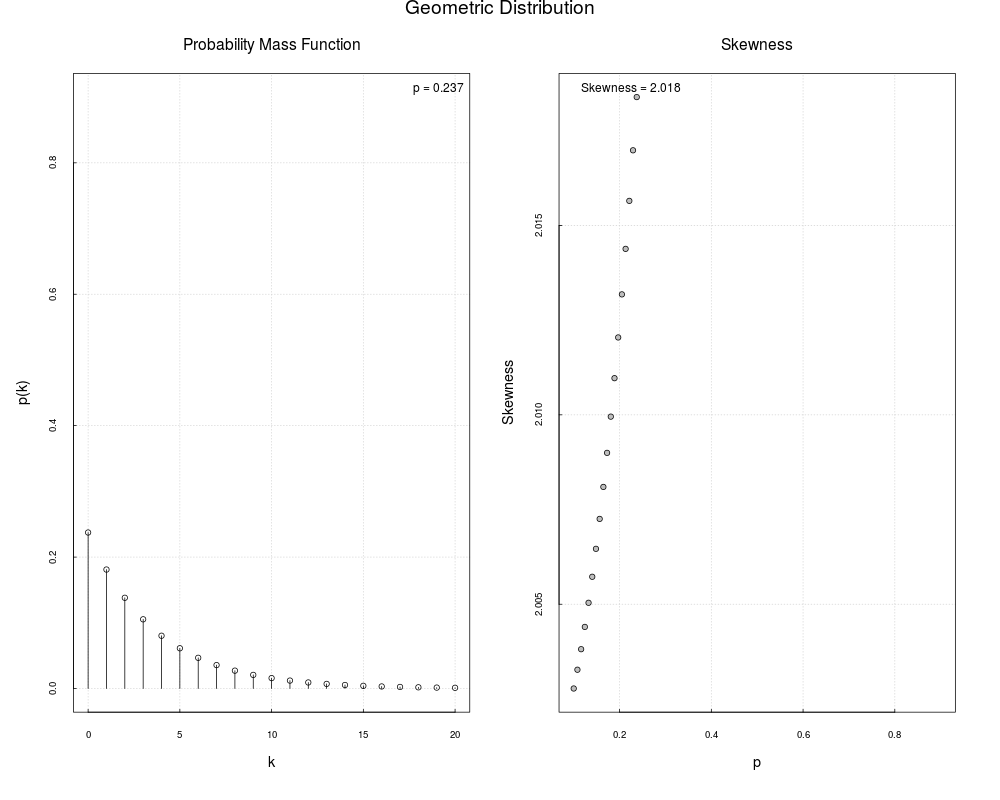
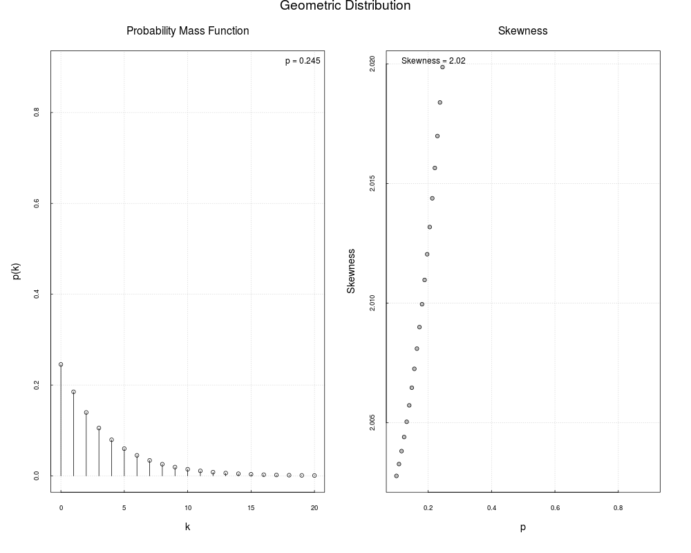
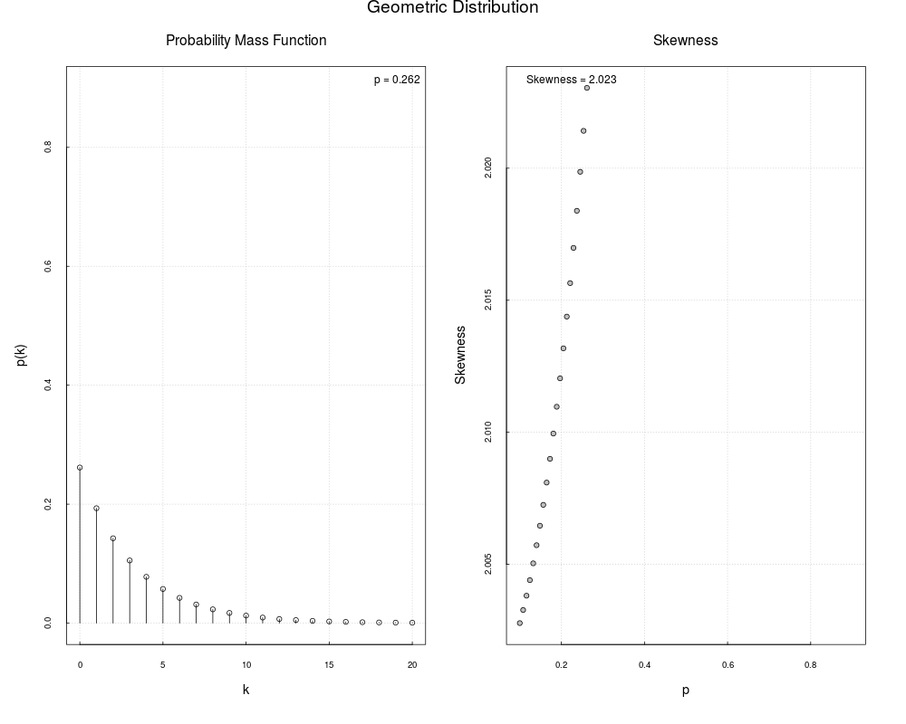
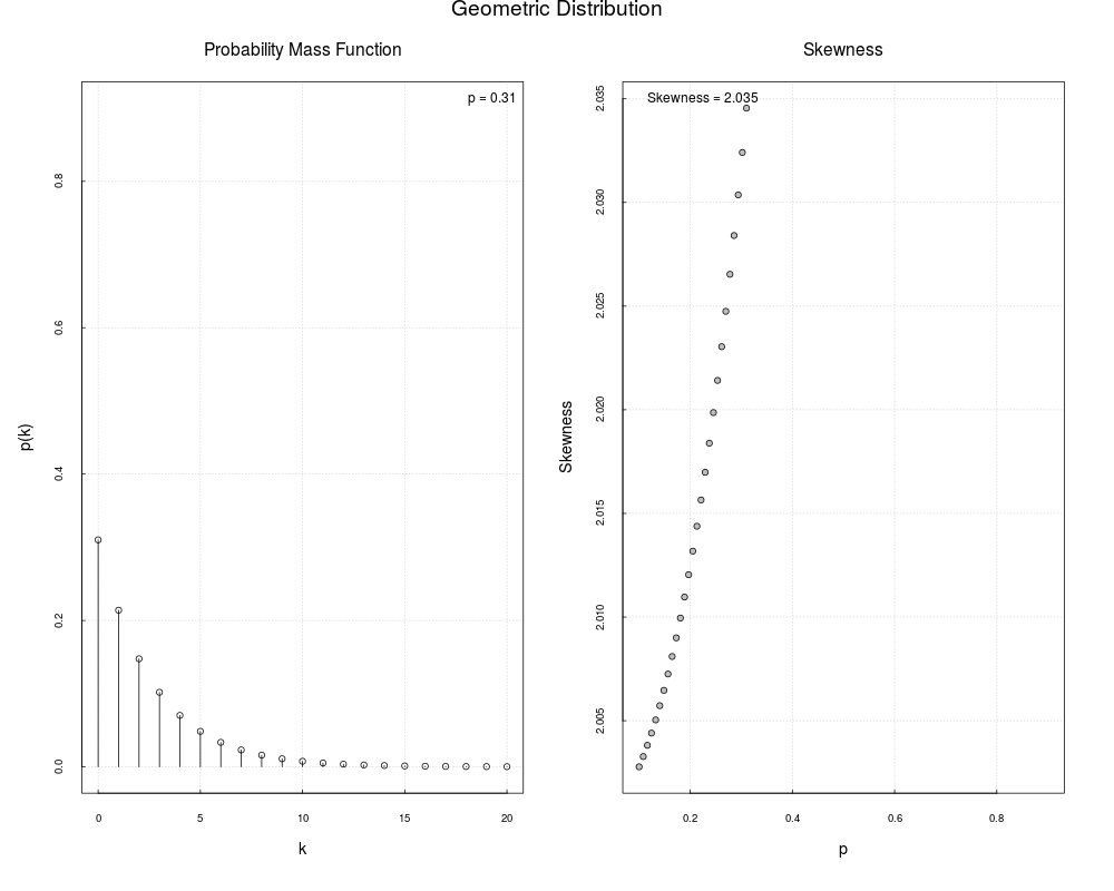
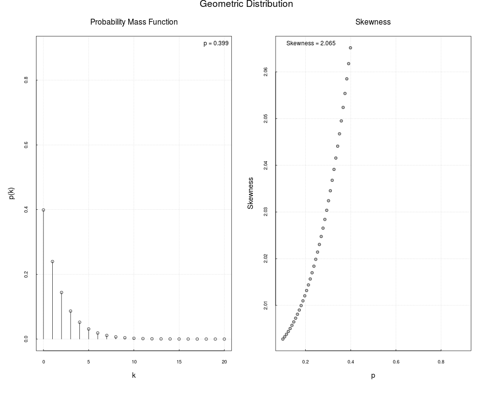
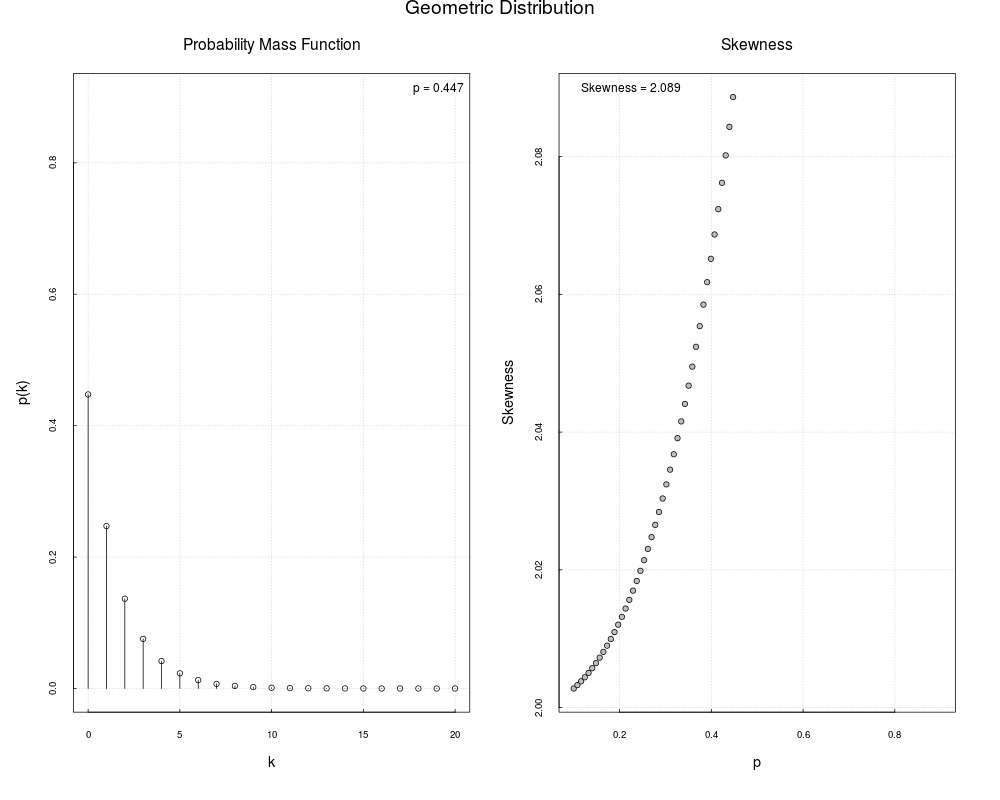
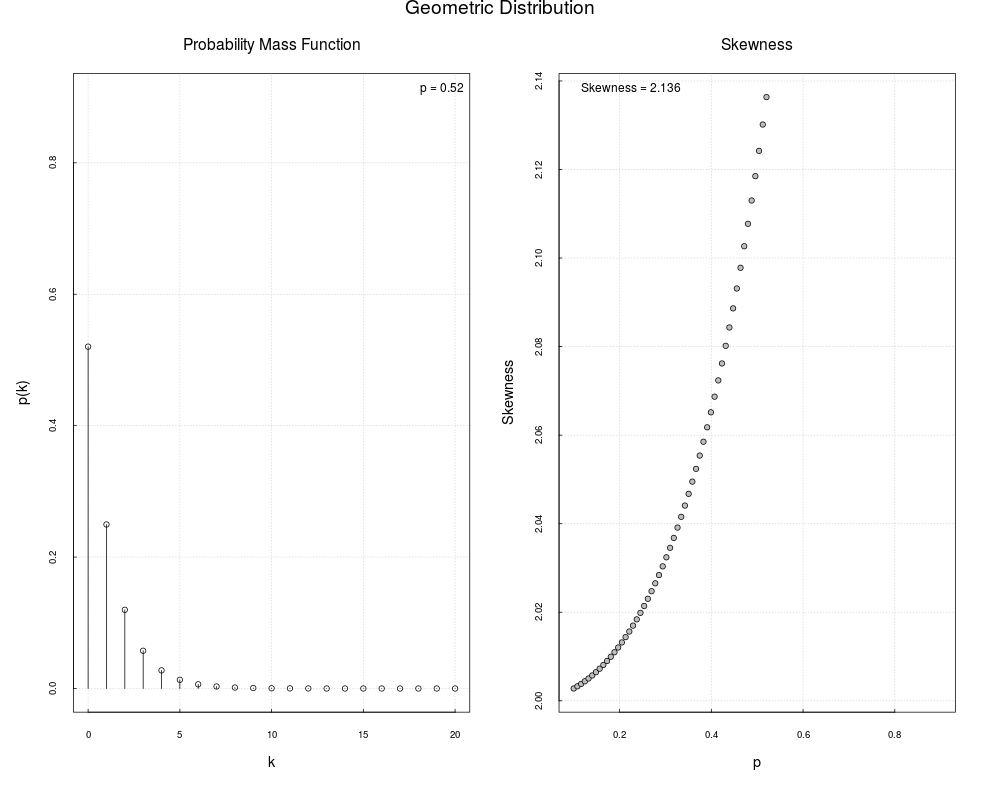
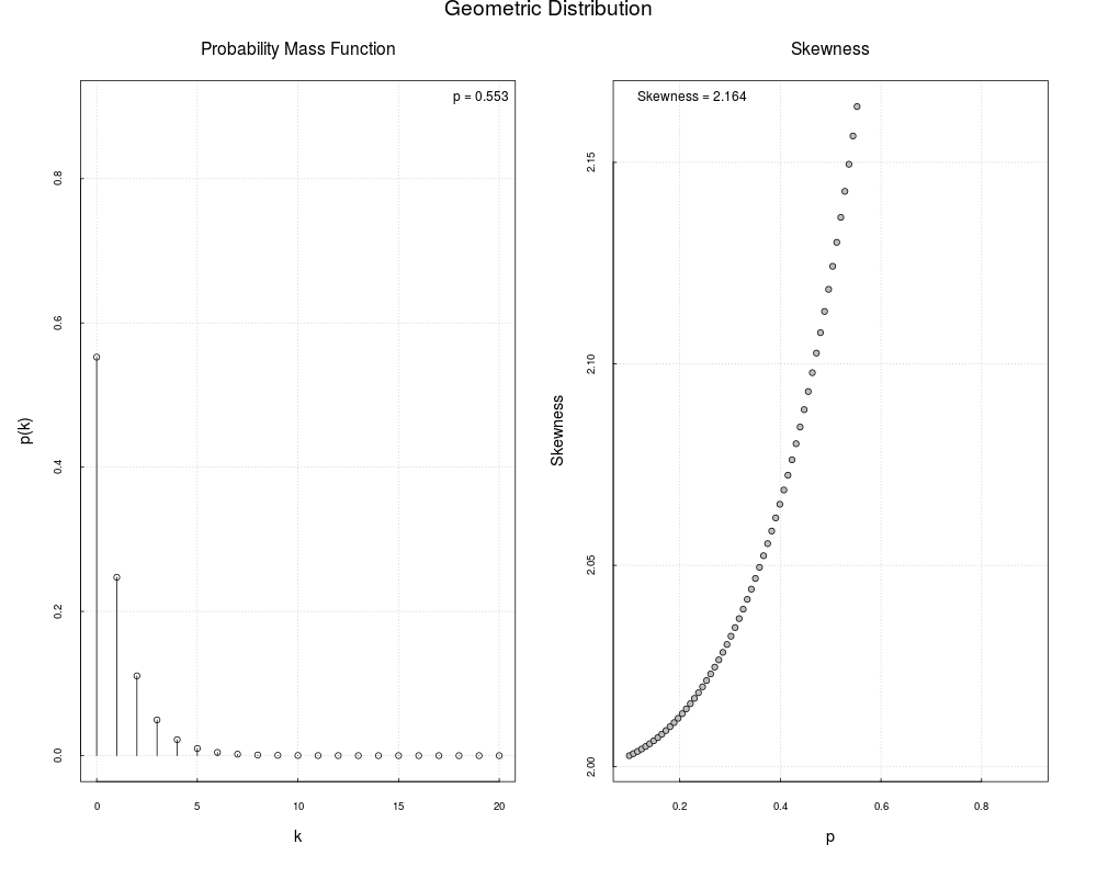
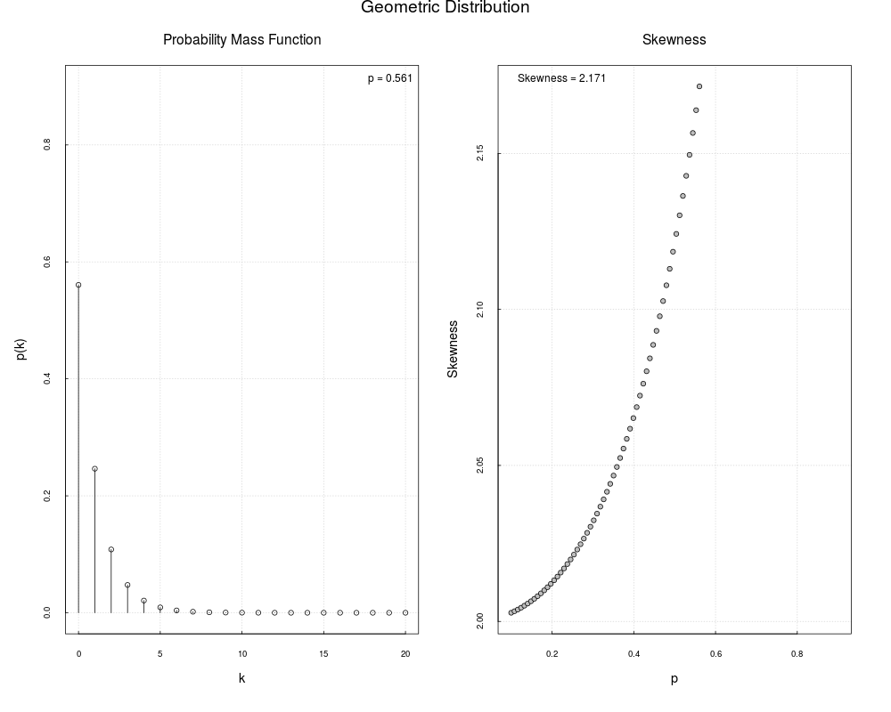
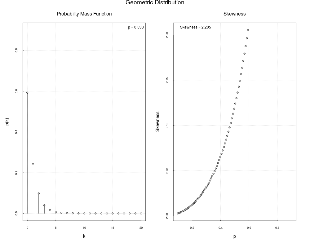
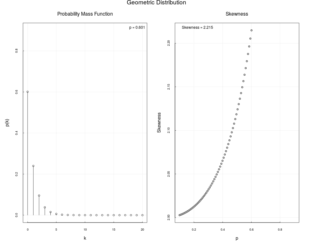
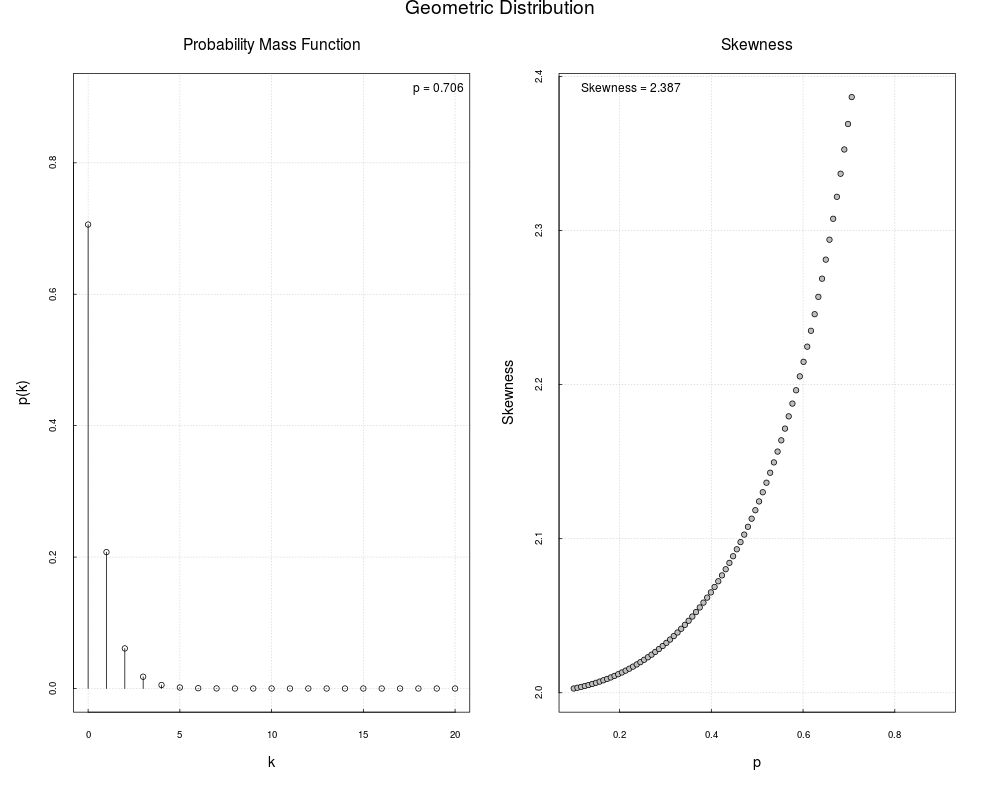
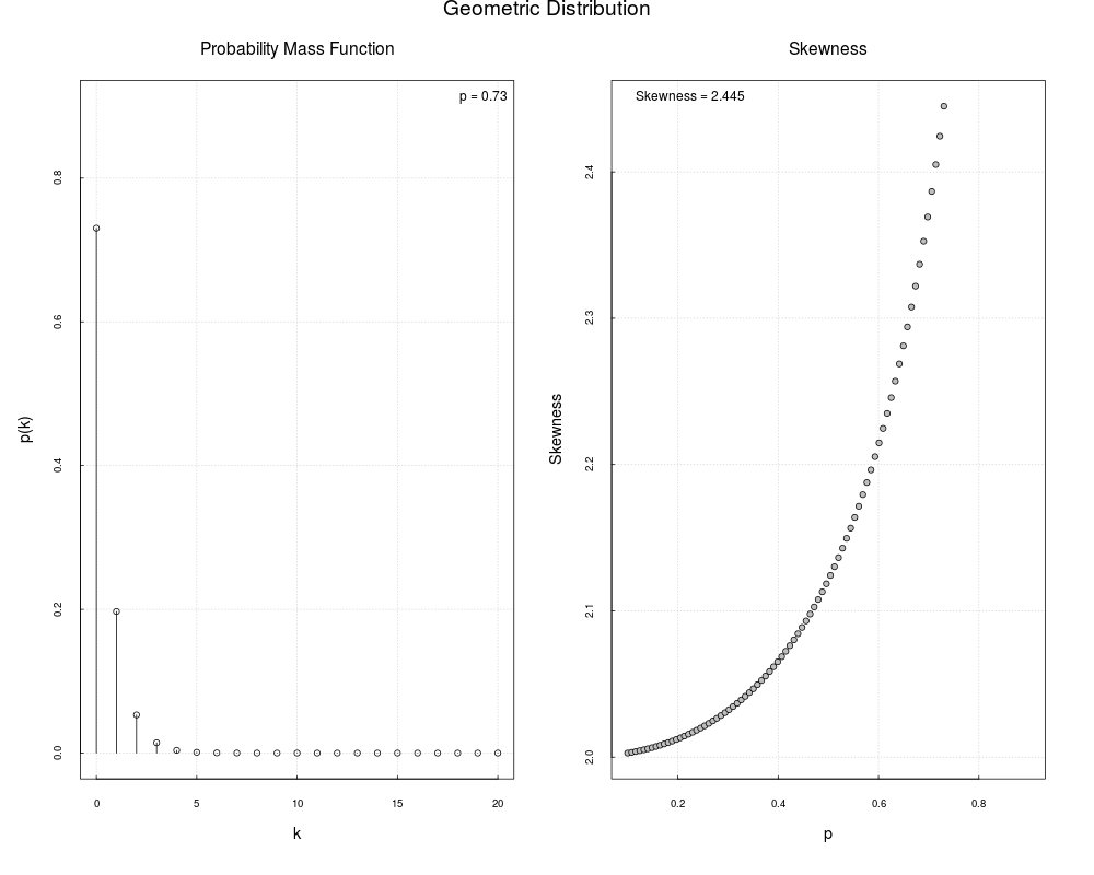
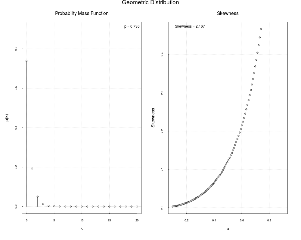
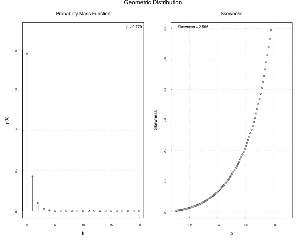
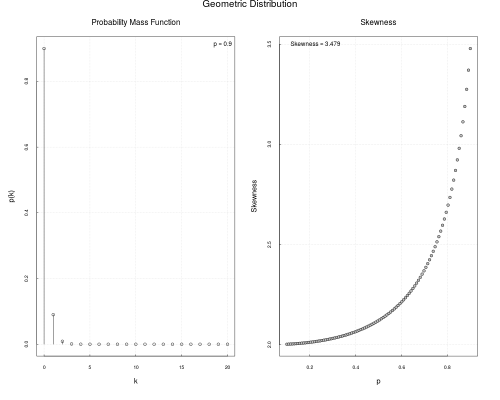
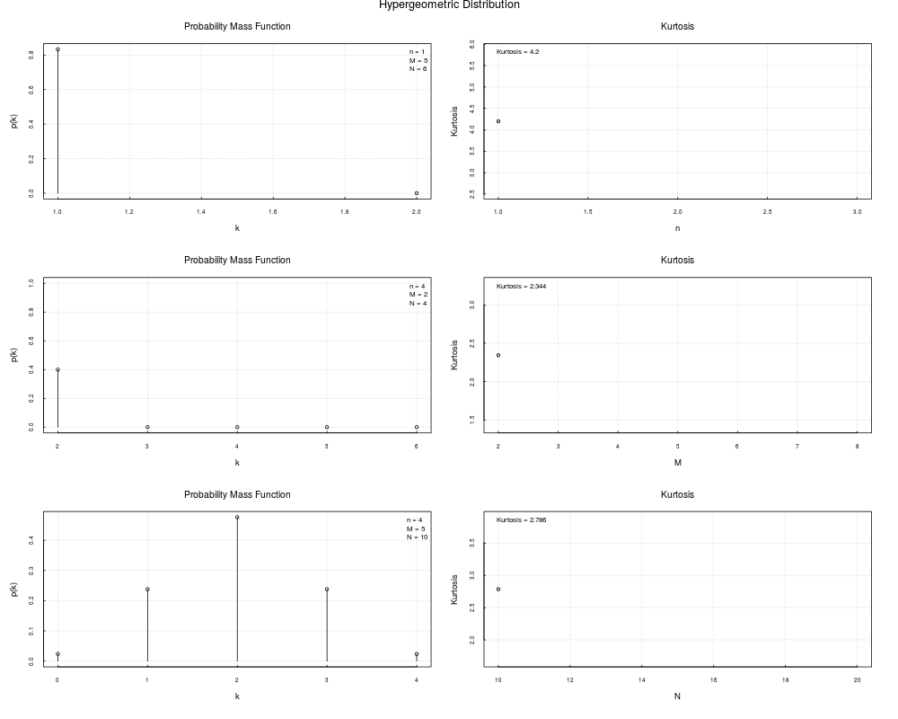
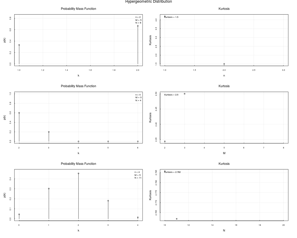
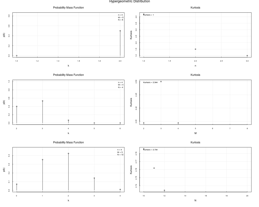
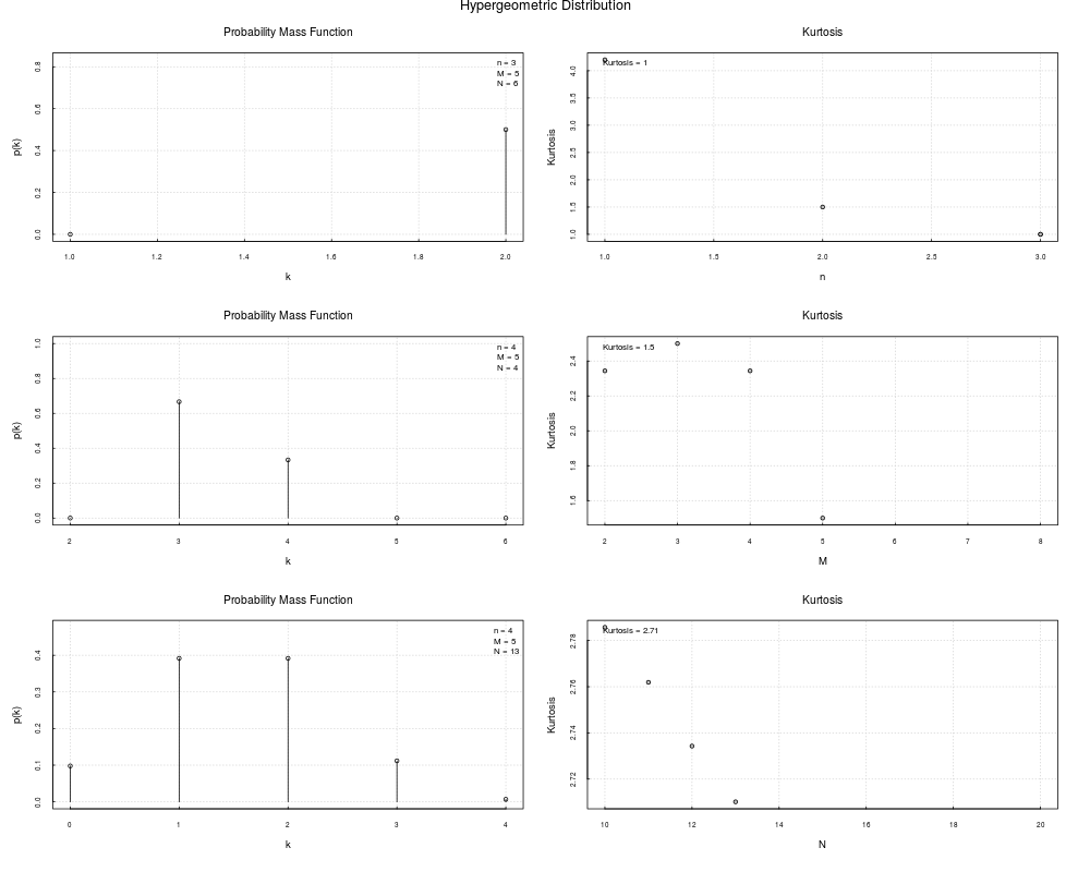
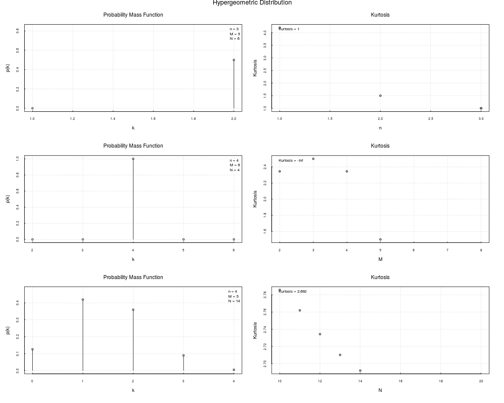
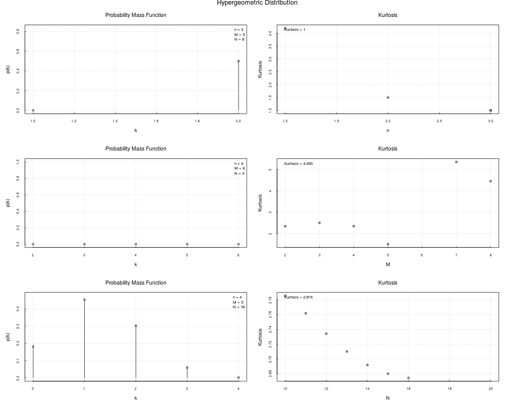
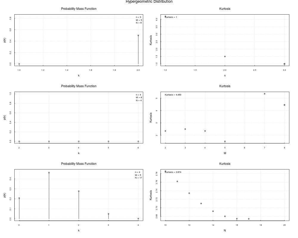
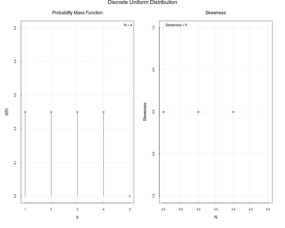
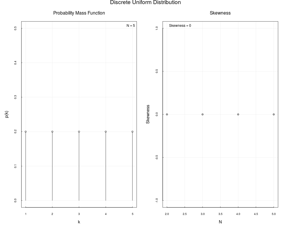
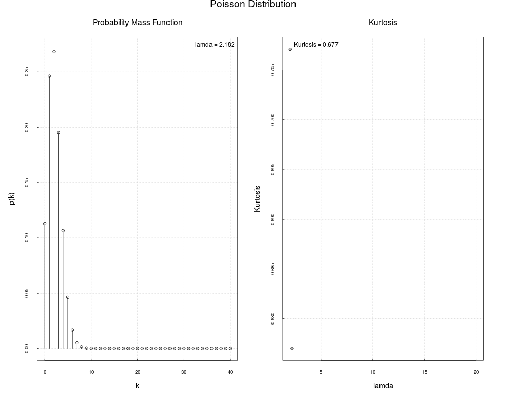
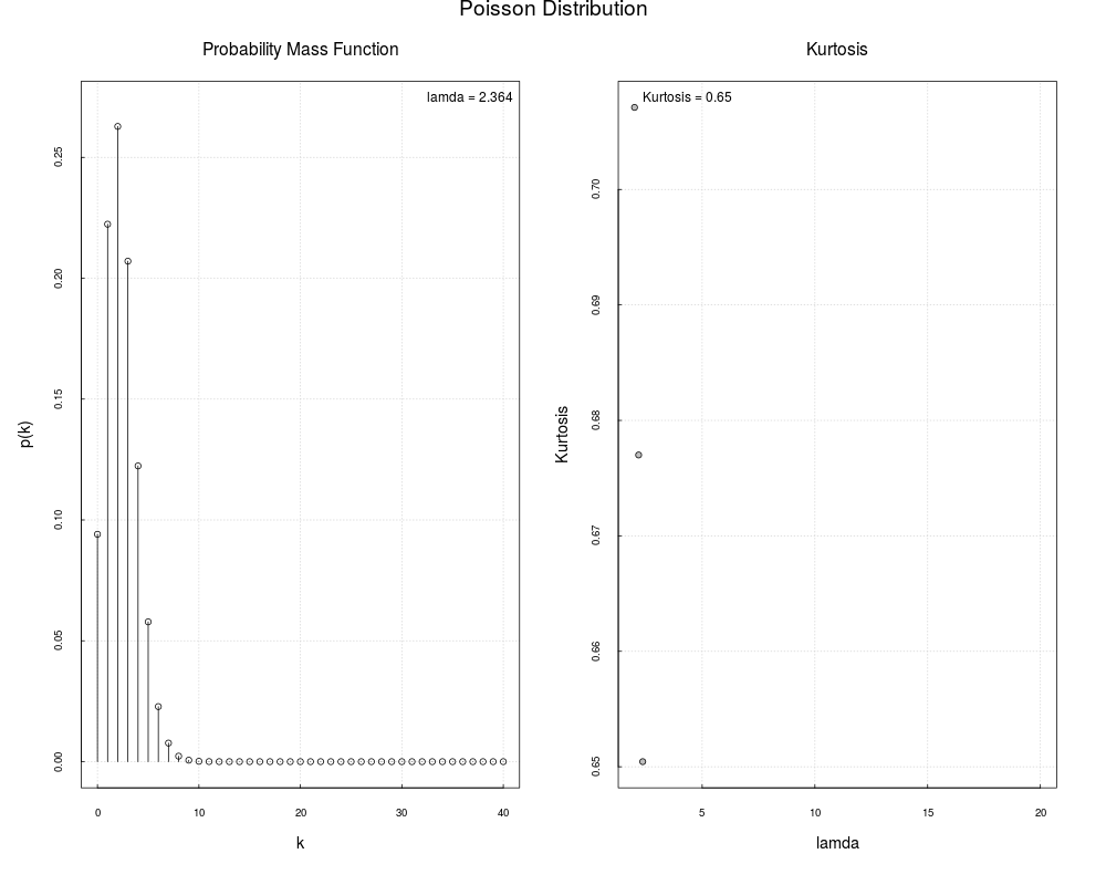
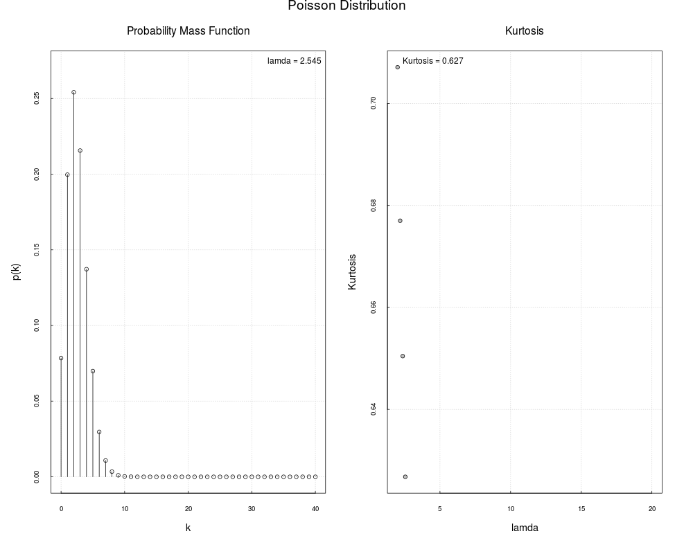
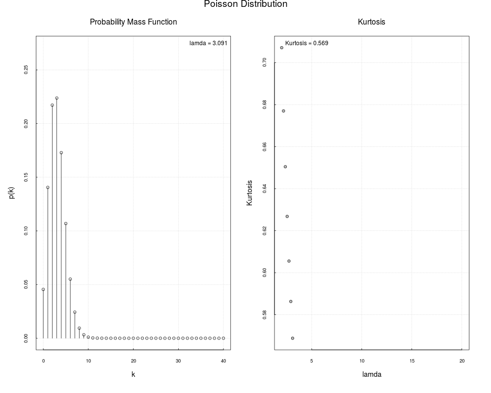
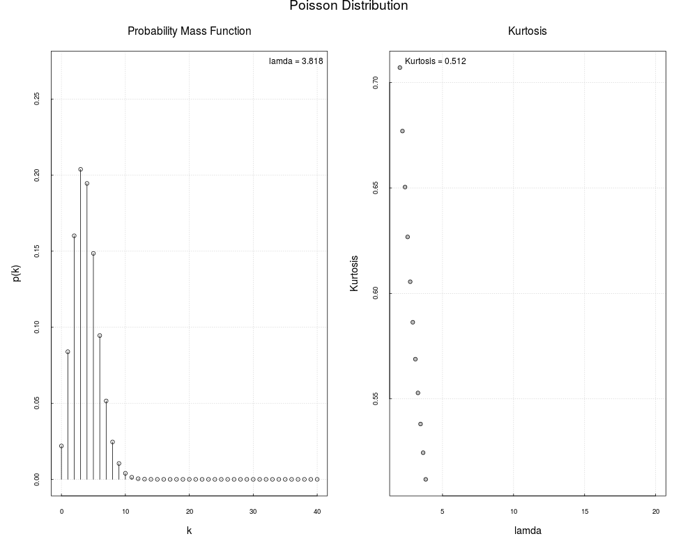
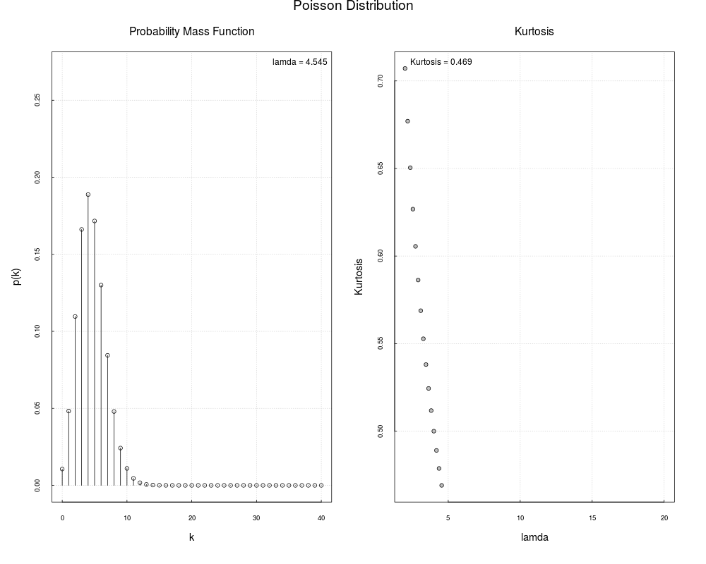
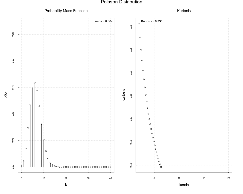
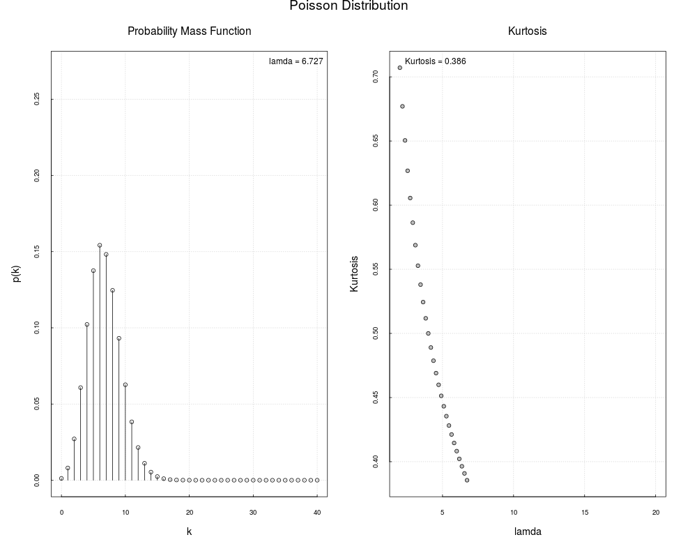
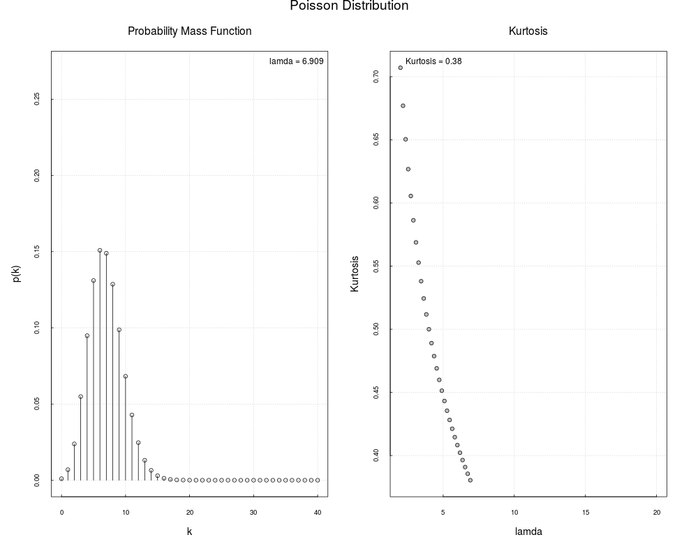
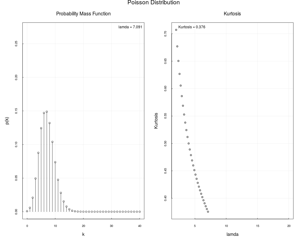
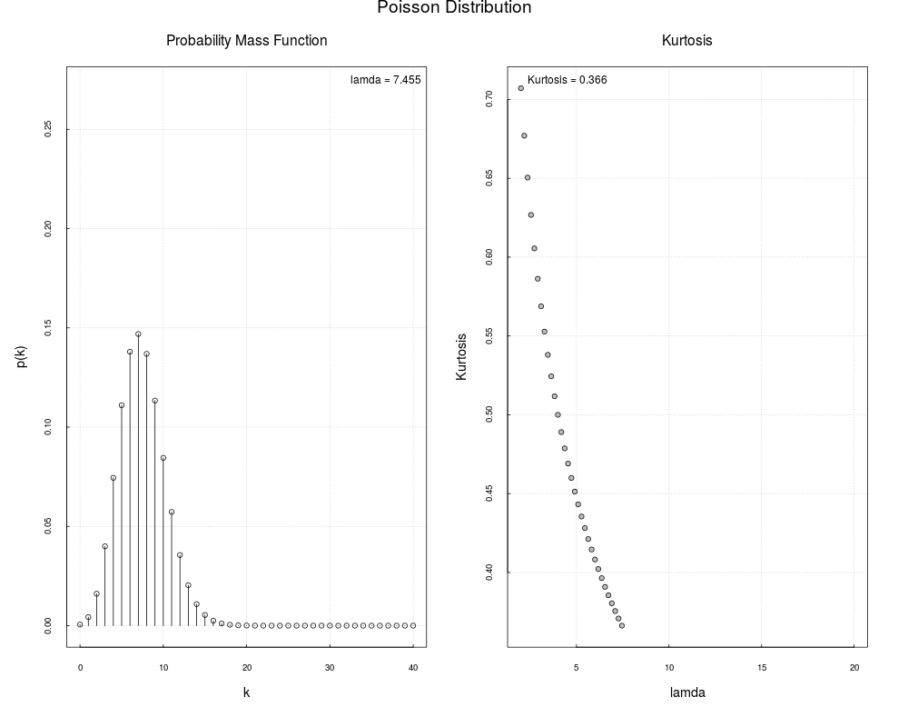
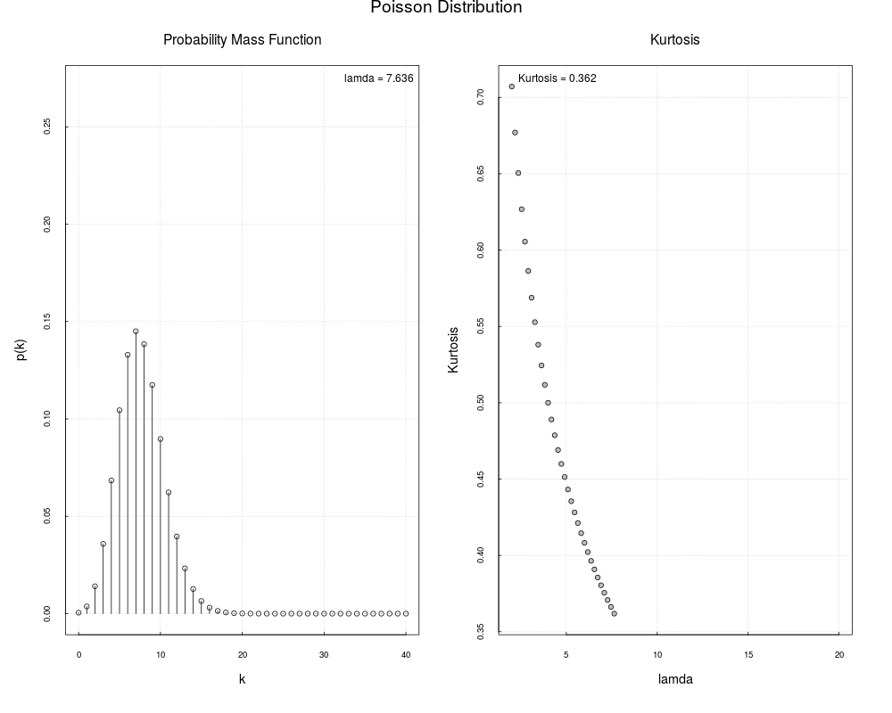
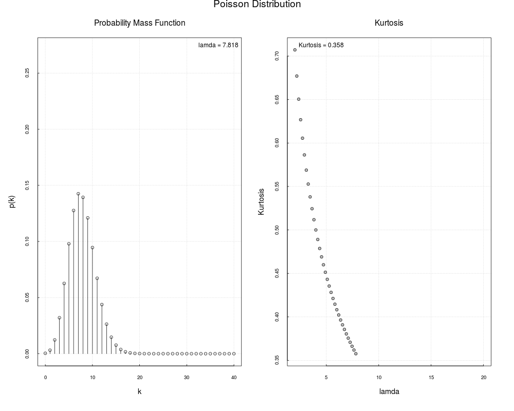
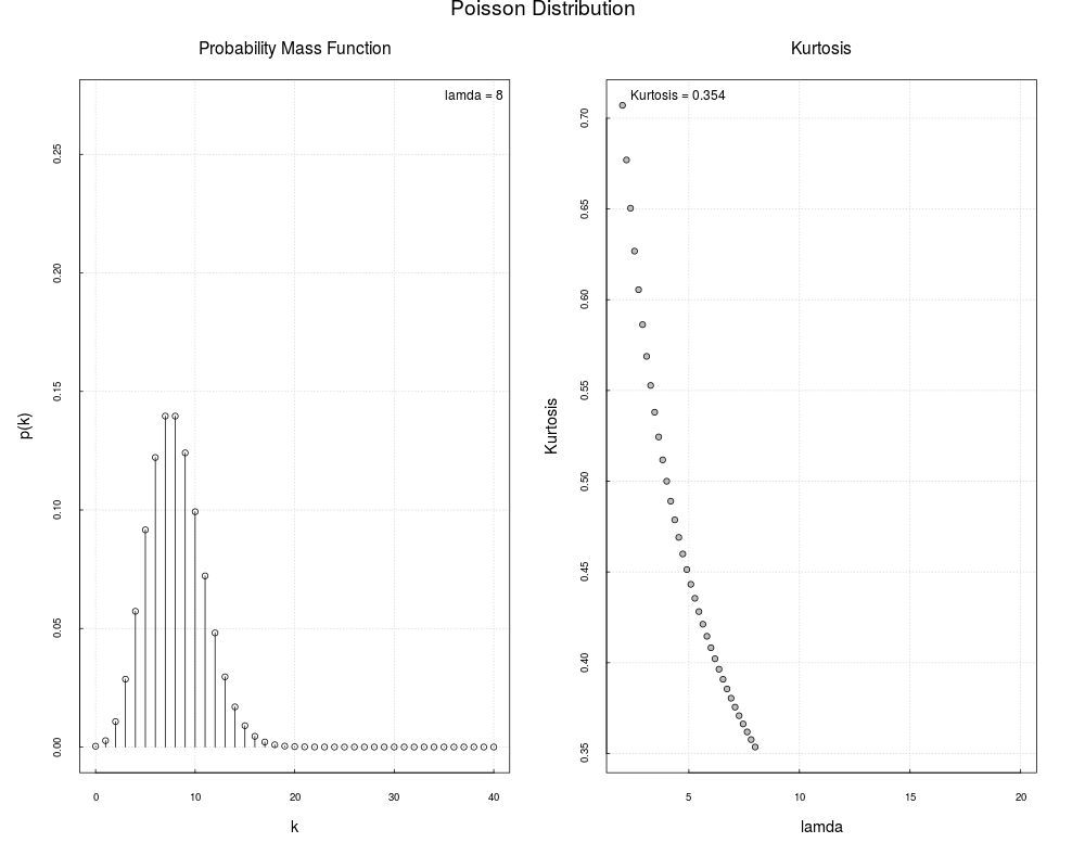
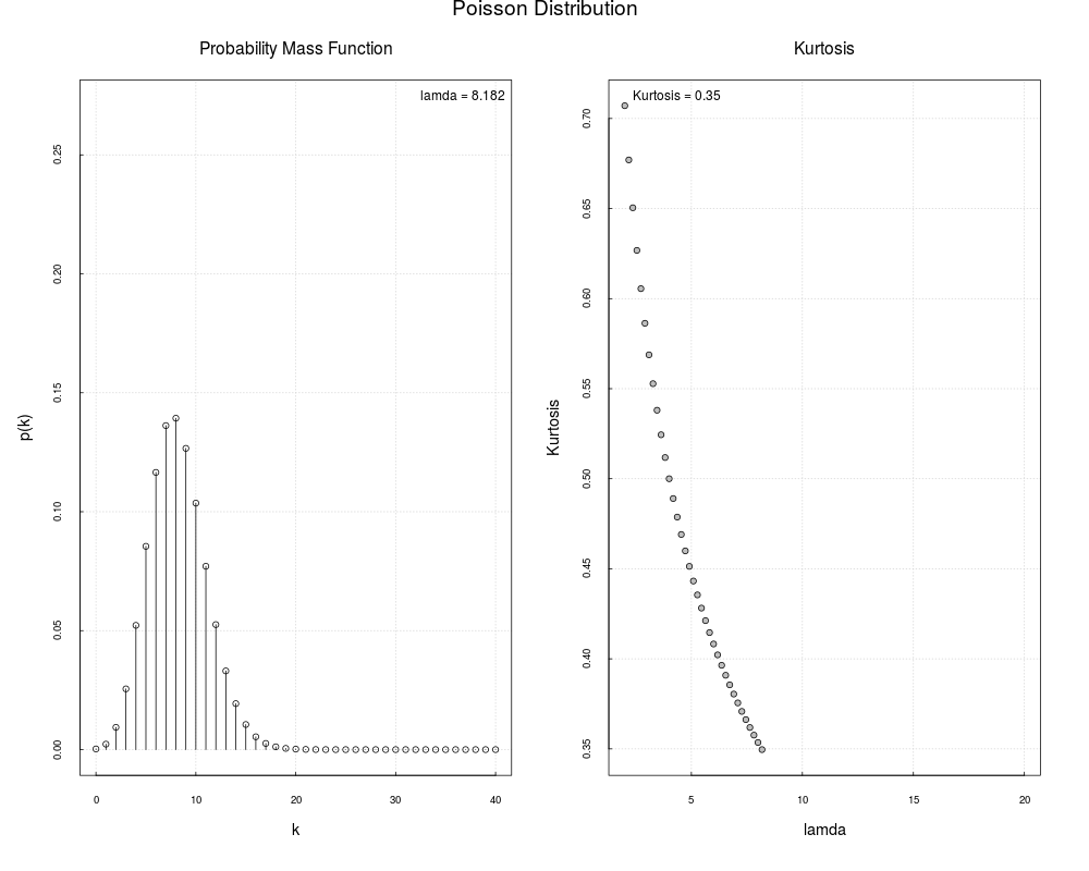
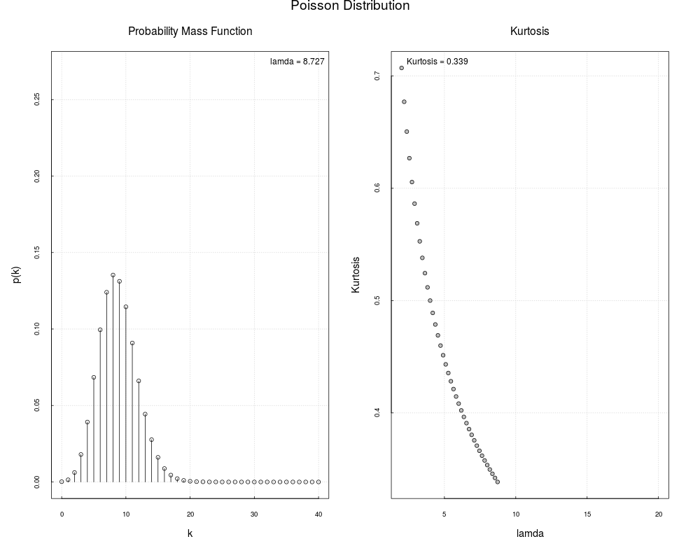
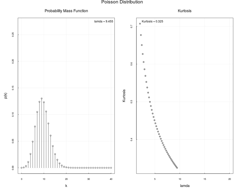
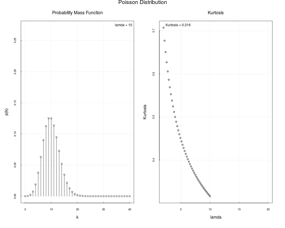
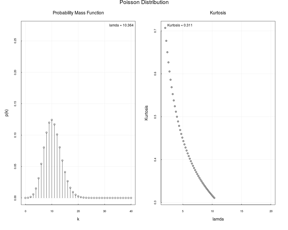
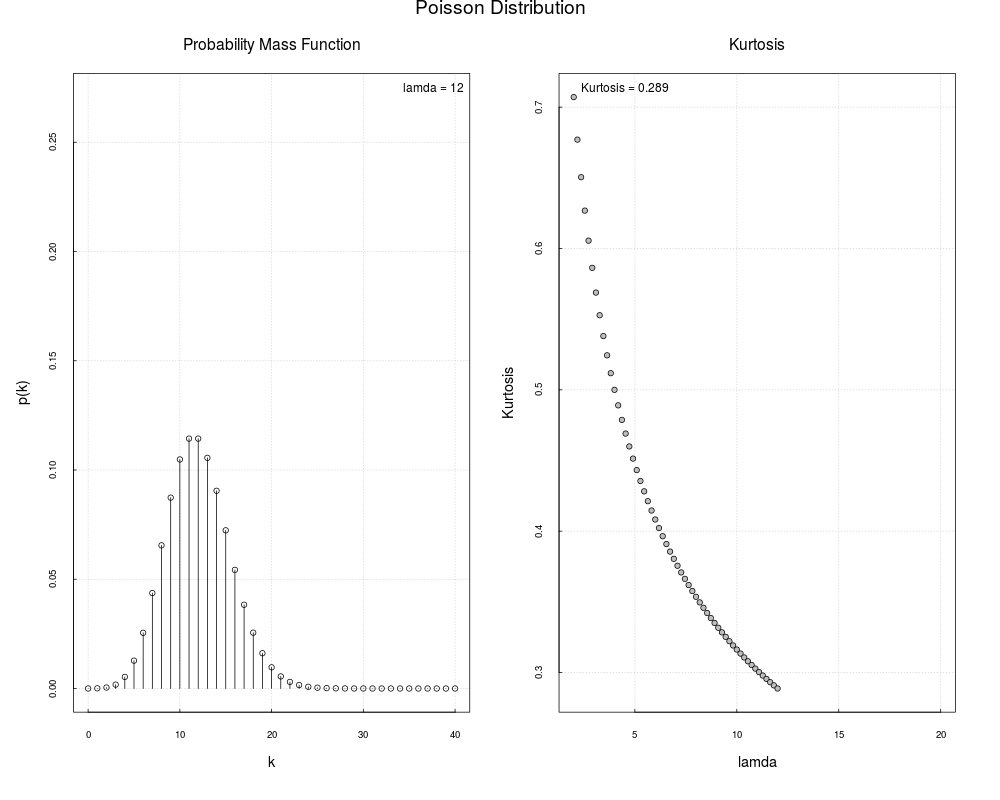
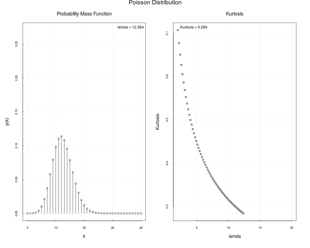
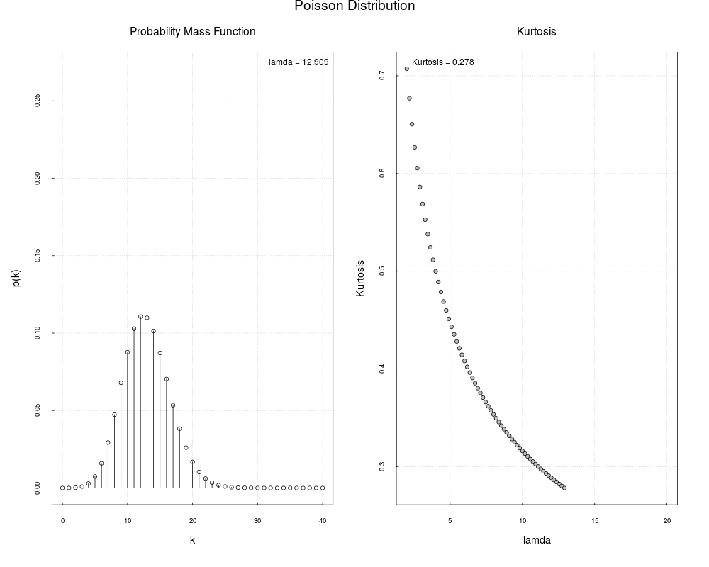
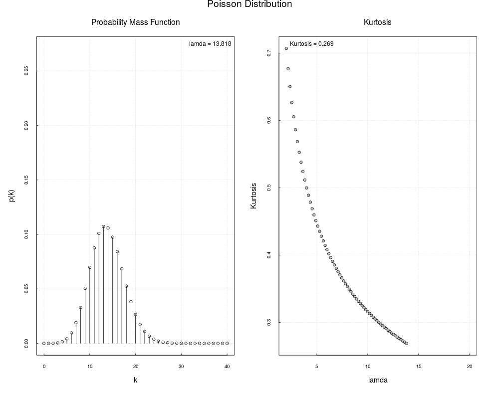
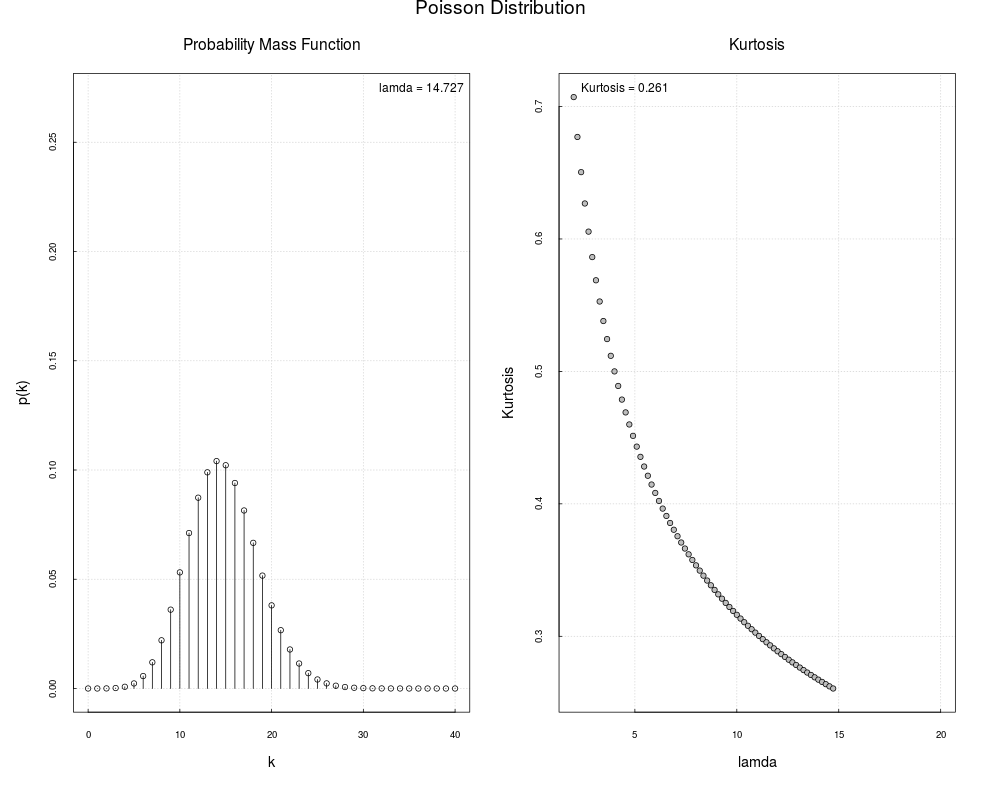
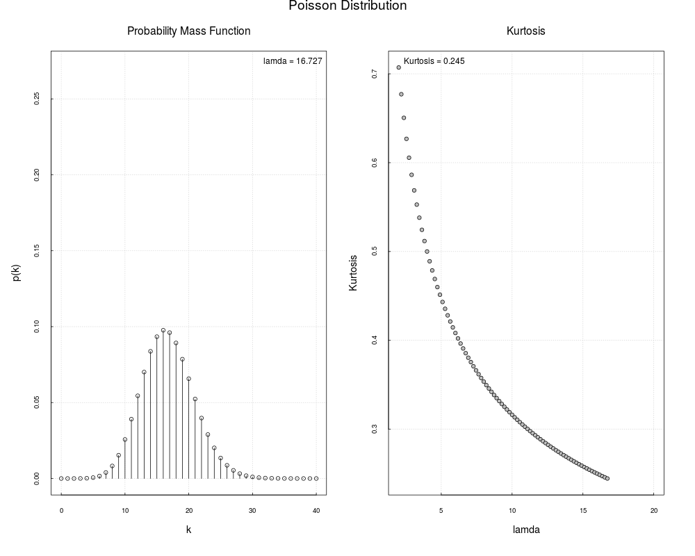
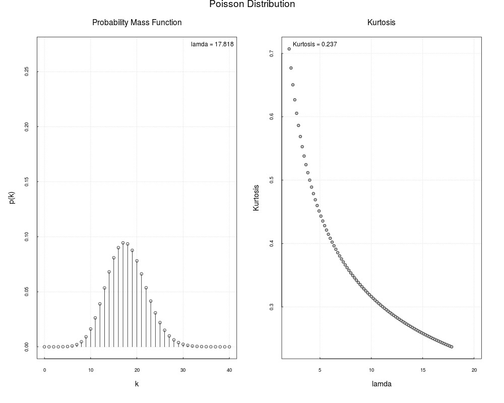
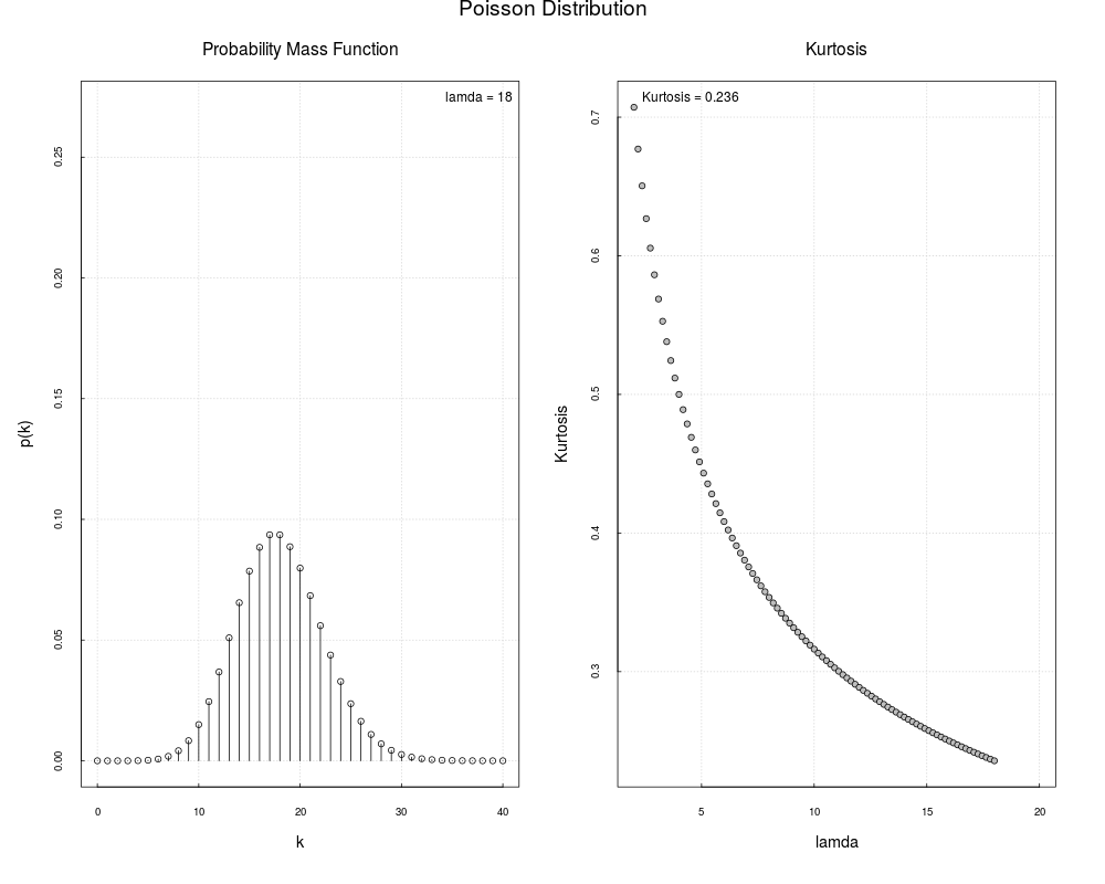
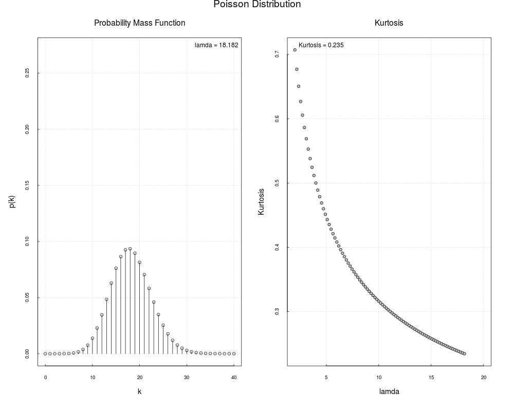
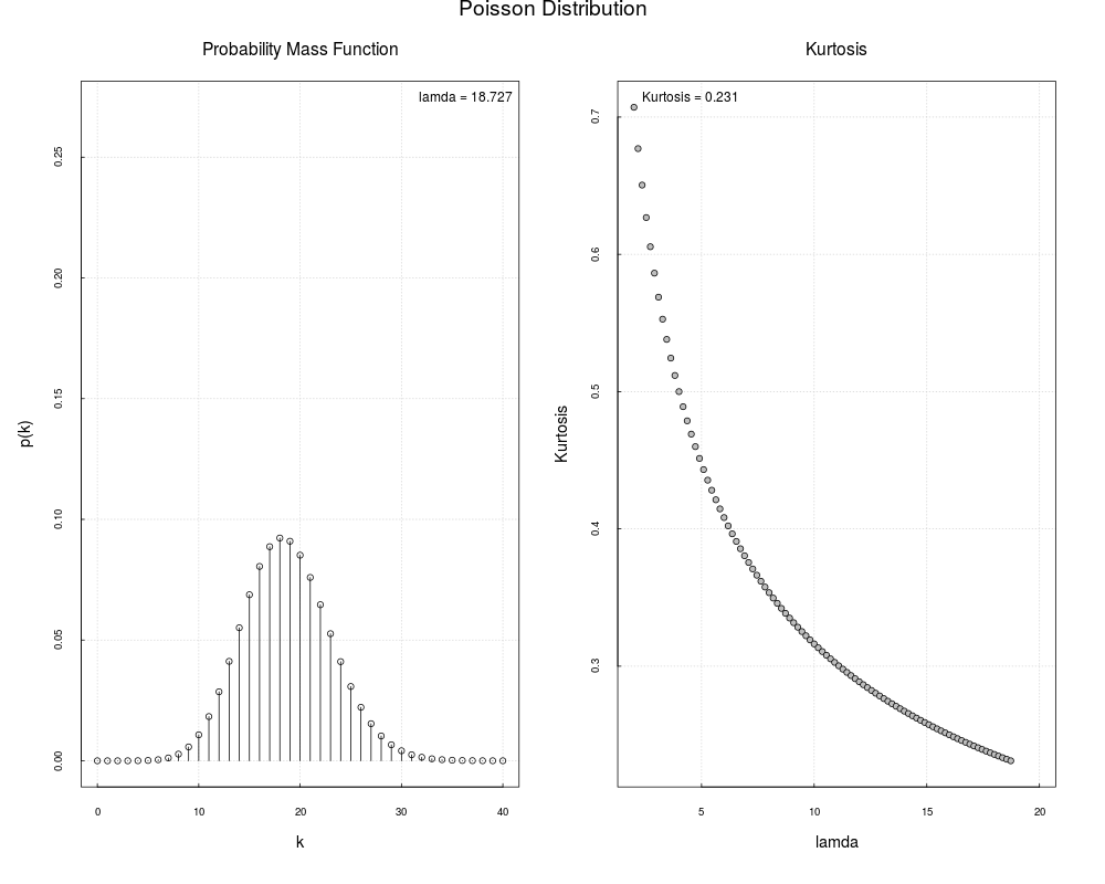
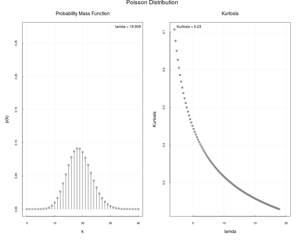
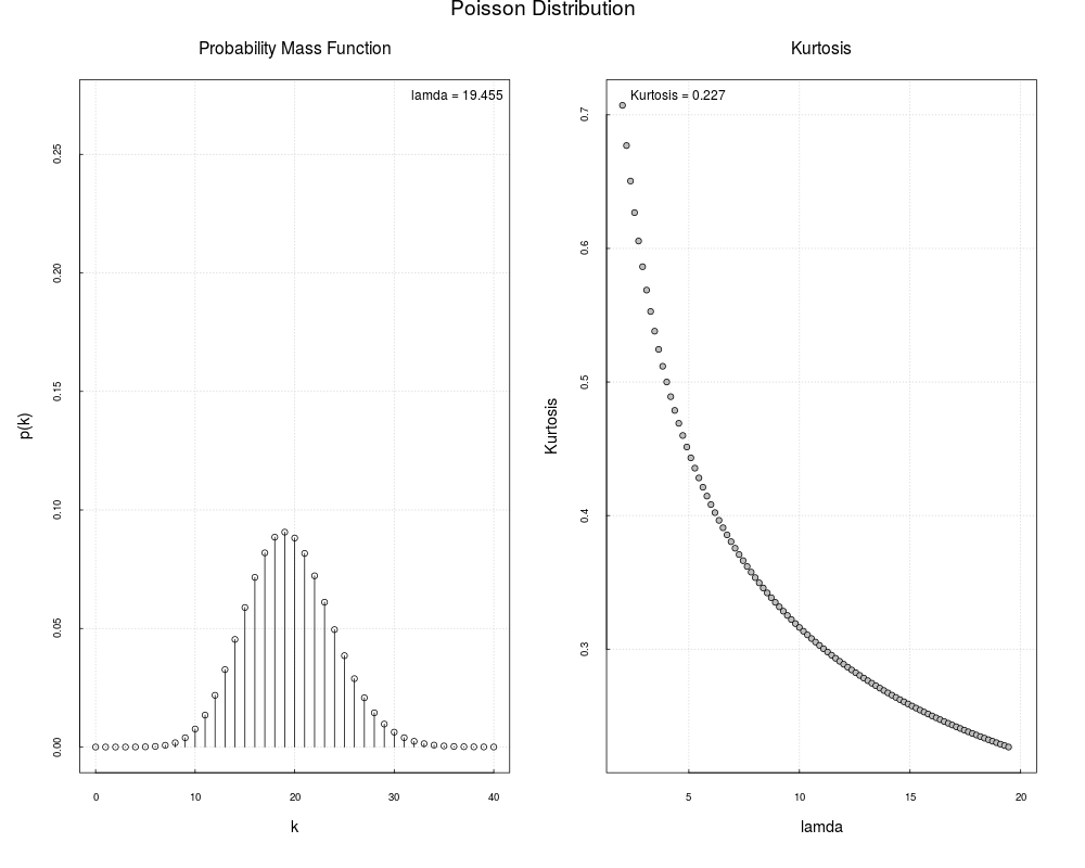
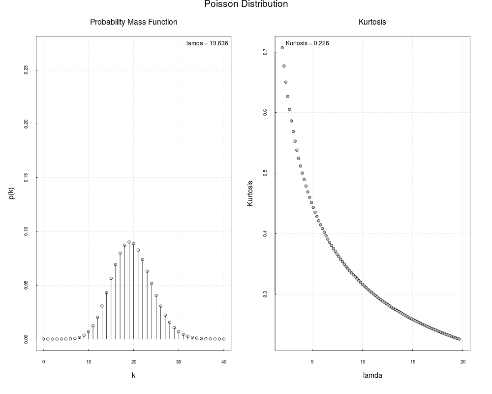
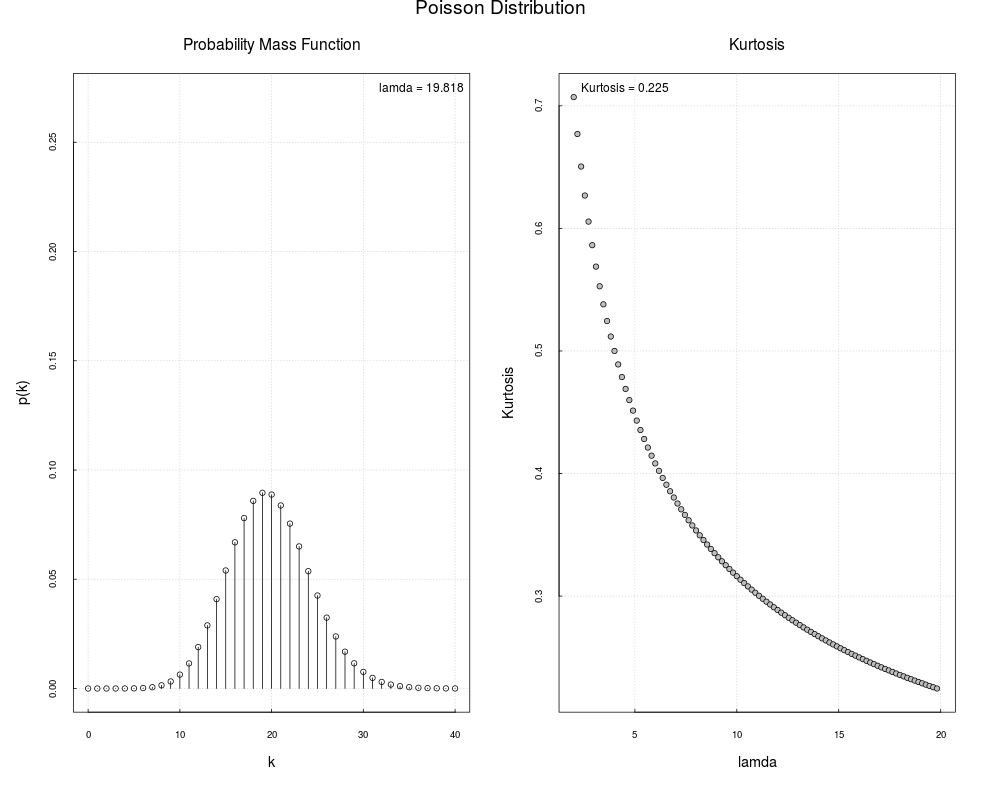
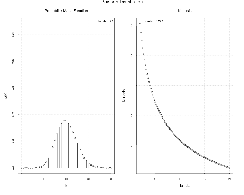
DetailsFor name, you can choose among Discrete Uniform('Dis_Uniform'), Bernoulli('Bernoulli'), Binomial('Binomial'), Hypergeometric('Hypergeometric'), Poisson('Poisson'), Geometric('Geometric'), Negative Binomial('Negative_Binomial'), Logarithmic Series('Logarithmic_Series'). For choice, you can choose among Cumulative Probability Function('cdf'), Mean('Mean'), Variance('Variance'), Mode('Mode'), Skewness('Skewness') and Kurtosis('Kurtosis'). More details about distributions and parameters are as follows: Bernoulli: Bernoulli distribution. The Bernoulli probability parameter is p, 0<p<1. Binomial: Binomial distribution. The Bernoulli trial parameter is n, and the probability parameter is p, 0<p<1.The order of parameters is: n, p. See Note below. Dis_Uniform: Discrete Uniform distribution. The parameter is n. Geometric: Geometric distribution. The Geometric trial parameter is n, and the probability parameter is p, 0<p<1. The order of parameters is: n, p. See Note below. Hypergeometric: Hypergeometric distribution. Parameter N: the number of elements in the population. Parameter M: the number of successes in the population. Parameter n: sample size. The order of parameters is N, M, n. See Note below. Logarithmic_Series: Logarithmic Series Distribution. Shape parameter theta, 0<theta <1.The probability function is (k*c^x)/x. For simplicity, let k =-1/log(1-c). Negative_Binomial: Negative Binomial distribution. The distribution of the random variable that represents the number of failures until the rth success is called geometric distribution. Parameter r: rth success.Parameter p: the Bernoulli probability parameter, 0<p<1.the order of parameters is r, p. See Note Below. Poisson: Poisson distribution. The parameter is lamda. ValueA dynamic graph which includes probability mass function graph and the 'choice' graph. NoteWhen you assign the parameter matrix to the argument par_matrix , you must follow the input sequence of parameters. Author(s)Lei ZHANG, Hao JIANG and Chen XUE (Equally contributed, the order is decided by the time the author joined the project.) ReferencesK. Krishnamoorthy(2006) Handbook of Statistical Distributions with Applications University of Louisiana at Lafayette. ExamplesDynDis(name=Negative_Binomial,par_matrix=matrix(c(1,12,0.1,0.9),2,2) ,choice='Kurtosis',const_par=c(4,0.7)) DynDis(name=Bernoulli,par_matrix=matrix(c(0.1,0.9),2,1),choice='cdf') DynDis(name=Binomial,par_matrix=matrix(c(1,12,0.1,0.9),2,2),choice='Mean' ,const_par=c(4,0.7)) DynDis(name=Logarithmic_Series,par_matrix=matrix(c(0.1,0.9),2,1), choice='Variance') DynDis(name=Geometric,par_matrix=matrix(c(0.1,0.9),2,1),choice='Skewness') DynDis(name=Hypergeometric,par_matrix=matrix(c(1,3,2,8,10,20),2,3), choice='Kurtosis',const_par=c(4,5,6)) DynDis(name=Dis_Uniform,par_matrix=matrix(c(2,5),2,1),choice='Skewness') DynDis(name=Poisson,par_matrix=matrix(c(2,20),2,1),choice='Kurtosis') Results
R version 3.3.1 (2016-06-21) -- "Bug in Your Hair"
Copyright (C) 2016 The R Foundation for Statistical Computing
Platform: x86_64-pc-linux-gnu (64-bit)

R is free software and comes with ABSOLUTELY NO WARRANTY.
You are welcome to redistribute it under certain conditions.
Type 'license()' or 'licence()' for distribution details.

R is a collaborative project with many contributors.
Type 'contributors()' for more information and
'citation()' on how to cite R or R packages in publications.

Type 'demo()' for some demos, 'help()' for on-line help, or
'help.start()' for an HTML browser interface to help.
Type 'q()' to quit R.

> library(DynamicDistribution)
> png(filename="/home/ddbj/snapshot/RGM3/R_CC/result/DynamicDistribution/DynDis.Rd_%03d_medium.png", width=480, height=480)
> ### Name: DynDis
> ### Title: Dynamically Visualized Discrete Probability Distributions and
> ###   Their Moments
> ### Aliases: DynDis
>
> ### ** Examples
>
> DynDis(name=Negative_Binomial,par_matrix=matrix(c(1,12,0.1,0.9),2,2)
+ ,choice='Kurtosis',const_par=c(4,0.7))
>
> DynDis(name=Bernoulli,par_matrix=matrix(c(0.1,0.9),2,1),choice='cdf')
>
> DynDis(name=Binomial,par_matrix=matrix(c(1,12,0.1,0.9),2,2),choice='Mean'
+ ,const_par=c(4,0.7))
>
> DynDis(name=Logarithmic_Series,par_matrix=matrix(c(0.1,0.9),2,1),
+ choice='Variance')
>
> DynDis(name=Geometric,par_matrix=matrix(c(0.1,0.9),2,1),choice='Skewness')
>
> DynDis(name=Hypergeometric,par_matrix=matrix(c(1,3,2,8,10,20),2,3),
+ choice='Kurtosis',const_par=c(4,5,6))
>
> DynDis(name=Dis_Uniform,par_matrix=matrix(c(2,5),2,1),choice='Skewness')
>
> DynDis(name=Poisson,par_matrix=matrix(c(2,20),2,1),choice='Kurtosis')
>
>
>
>
>
> dev.off()
null device
          1
>
|