Plotting function for ensemble models of the class "FDatFitLogit" or "FDatFitNormal", which are the objects created by the calibrateEnsemble() function.

Description

Default plotting for objectes created by the "calibrateEnsemble" function. See details below.

Usage

## S4 method for signature 'FDatFitLogit'
plot(x, period = "calibration", subset = 1,
  mainLabel = "", xLab = "", yLab = "", cols = 1, ...)

Arguments

Details

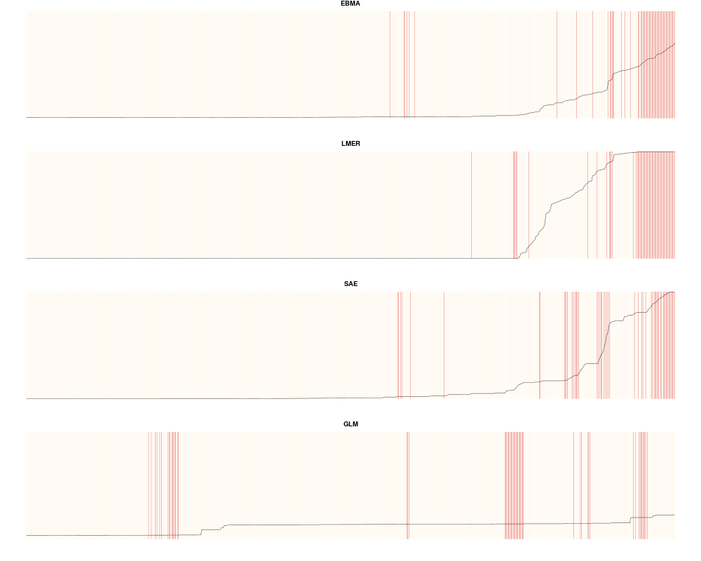
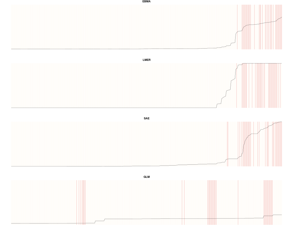
For objects of the class "FDatFitLogit", this function creates separation plots for each of the fitted models, including the EBMA model. Observations are ordered from left to right with increasing predicted probabilities, which is depicted by the black line. Actual occurrences are displayed by red vertical lines. Plots can be displayed for the test or calibration period. For objects of the class "FDatFitNormal", this function creates a plot of the predictive density distribution containing the EBMA PDF and the PDFs for all component models (scaled by their model weights). It also plots the prediction for the ensemble and the components for the specified observations.

Author(s)

Michael D. Ward <michael.d.ward@duke.edu> and Jacob M. Montgomery <jacob.montgomery@wustl.edu> and Florian M. Hollenbach <florian.hollenbach@tamu.edu>

References

Raftery, A. E., T. Gneiting, F. Balabdaoui and M. Polakowski. (2005). Using Bayesian Model Averaging to calibrate forecast ensembles. Monthly Weather Review. 133:1155–1174.

Greenhill, B., M.D. Ward, A. Sacks. (2011). The Separation Plot: A New Visual Method For Evaluating the Fit of Binary Data. American Journal of Political Science.55: 991–1002.

Montgomery, Jacob M., Florian M. Hollenbach and Michael D. Ward. (2012). Improving Predictions Using Ensemble Bayesian Model Averaging. Political Analysis. 20: 271-291.

Montgomery, Jacob M., Florian M. Hollenbach and Michael D. Ward. (2015). Calibrating ensemble forecasting models with sparse data in the social sciences. International Journal of Forecasting. In Press.

See Also

separationplot

Examples

data(calibrationSample)

data(testSample) 

this.ForecastData <- makeForecastData(.predCalibration=calibrationSample[,c("LMER", "SAE", "GLM")],
.outcomeCalibration=calibrationSample[,"Insurgency"],.predTest=testSample[,c("LMER", "SAE", "GLM")],
.outcomeTest=testSample[,"Insurgency"], .modelNames=c("LMER", "SAE", "GLM"))

this.ensemble <- calibrateEnsemble(this.ForecastData, model="logit", tol=0.001, exp=3)

plot(this.ensemble, period="calibration") 
plot(this.ensemble, period="test")

Results

R version 3.3.1 (2016-06-21) -- "Bug in Your Hair"
Copyright (C) 2016 The R Foundation for Statistical Computing
Platform: x86_64-pc-linux-gnu (64-bit)

R is free software and comes with ABSOLUTELY NO WARRANTY.
You are welcome to redistribute it under certain conditions.
Type 'license()' or 'licence()' for distribution details.

R is a collaborative project with many contributors.
Type 'contributors()' for more information and
'citation()' on how to cite R or R packages in publications.

Type 'demo()' for some demos, 'help()' for on-line help, or
'help.start()' for an HTML browser interface to help.
Type 'q()' to quit R.

> library(EBMAforecast)
Loading required package: separationplot
Loading required package: plyr
Loading required package: Hmisc
Loading required package: lattice
Loading required package: survival
Loading required package: Formula
Loading required package: ggplot2

Attaching package: 'Hmisc'

The following objects are masked from 'package:plyr':

    is.discrete, summarize

The following objects are masked from 'package:base':

    format.pval, round.POSIXt, trunc.POSIXt, units

Loading required package: abind
> png(filename="/home/ddbj/snapshot/RGM3/R_CC/result/EBMAforecast/plot-FDatFitLogit-method.Rd_%03d_medium.png", width=480, height=480)
> ### Name: plot,FDatFitLogit-method
> ### Title: Plotting function for ensemble models of the class
> ###   "FDatFitLogit" or "FDatFitNormal", which are the objects created by
> ###   the 'calibrateEnsemble()' function.
> ### Aliases: plot,FDatFitLogit-method plot,FDatFitNormal-method
> 
> ### ** Examples
> 
> data(calibrationSample)
> 
> data(testSample) 
> 
> this.ForecastData <- makeForecastData(.predCalibration=calibrationSample[,c("LMER", "SAE", "GLM")],
+ .outcomeCalibration=calibrationSample[,"Insurgency"],.predTest=testSample[,c("LMER", "SAE", "GLM")],
+ .outcomeTest=testSample[,"Insurgency"], .modelNames=c("LMER", "SAE", "GLM"))
> 
> this.ensemble <- calibrateEnsemble(this.ForecastData, model="logit", tol=0.001, exp=3)
> 
> plot(this.ensemble, period="calibration") 
> plot(this.ensemble, period="test")
> 
> 
> 
> 
> 
> 
> dev.off()
null device 
          1 
>