R Graphical Manual

Browse All

Last data update: 2014.03.03

R: Function to evaluate the initial cumulative explained...

test.factors

R Documentation

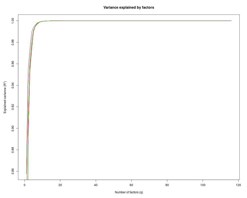
Function to evaluate the initial cumulative explained variance.

Description

This function performs eigenspace decomposition using the weight-transformed matrix W to determine the minimum number of end-members. Depending on the number of provided weight transformation limits (l) a single vector or a matrix is returned.

Usage

test.factors(X, l, c, r.min = 0.95, plot = FALSE, legend, ..., pm = FALSE)

Arguments

`X`	Numeric matrix with m samples (rows) and n variables (columns).
`l`	Numeric vector specifying the weight tranformation limits, i.e. quantiles; default is 0.
`c`	Numeric scalar specifying the constant sum scaling parameter, e.g. 1, 100, 1000; default is 100.
`r.min`	Numeric scalar, minimum value of explained variance to be reached by the end-members included, default is 0.95.
`plot`	Logical scalar, optional graphical output of the results, default is FALSE.,
`legend`	Character scalar, specify legend position (cf. `legend`). If omitted, no legend will be plotted, default is no legend.
`pm`	Logical scalar to enable pm.
`...`	Additional arguments passed to the plot function. Use `colour` instead of `col` to create different colours.

Details

The results may be used to define a minimum number of end-members for subsequent modelling steps, e.g. by using the Kaiser criterion, which demands a minimum number of eigenvalues to reach a squared R of 0.95.

Value

A list with objects

`L`	Vector or matrix of cumulative explained variance.
`q.min`	Vector with number of factors that passed r.min.

Author(s)

Michael Dietze, Elisabeth Dietze

References

Dietze E, Hartmann K, Diekmann B, IJmker J, Lehmkuhl F, Opitz S, Stauch G, Wuennemann B, Borchers A. 2012. An end-member algorithm for deciphering modern detrital processes from lake sediments of Lake Donggi Cona, NE Tibetan Plateau, China. Sedimentary Geology 243-244: 169-180.

Examples

## load example data set
data(X, envir = environment())

## create sequence of weight transformation limits
l <- seq(from = 0, to = 0.2, 0.02)

## perform the test and show q.min
L <- test.factors(X = X, l = l, c = 100, plot = TRUE)
L$q.min

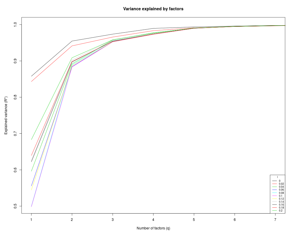
## a visualisation with more plot parameters
L <- test.factors(X = X, l = l, c = 100, plot = TRUE,
                  ylim = c(0.5, 1), xlim = c(1, 7),
                  legend = "bottomright", cex = 0.7)

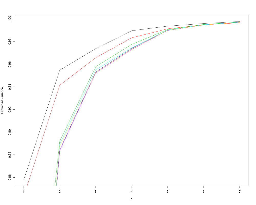
## another visualisation, a close-up
plot(1:7, L$L[1,1:7], type = "l",
     xlab = "q", ylab = "Explained variance")
for(i in 2:7) {lines(1:7, L$L[i,1:7], col = i)}

Results


R version 3.3.1 (2016-06-21) -- "Bug in Your Hair"
Copyright (C) 2016 The R Foundation for Statistical Computing
Platform: x86_64-pc-linux-gnu (64-bit)

R is free software and comes with ABSOLUTELY NO WARRANTY.
You are welcome to redistribute it under certain conditions.
Type 'license()' or 'licence()' for distribution details.

R is a collaborative project with many contributors.
Type 'contributors()' for more information and
'citation()' on how to cite R or R packages in publications.

Type 'demo()' for some demos, 'help()' for on-line help, or
'help.start()' for an HTML browser interface to help.
Type 'q()' to quit R.

> library(EMMAgeo)
Loading required package: GPArotation
Loading required package: limSolve
Loading required package: shape
Loading required package: shiny
> png(filename="/home/ddbj/snapshot/RGM3/R_CC/result/EMMAgeo/test.factors.Rd_%03d_medium.png", width=480, height=480)
> ### Name: test.factors
> ### Title: Function to evaluate the initial cumulative explained variance.
> ### Aliases: test.factors
> ### Keywords: EMMA
> 
> ### ** Examples
> 
> ## load example data set
> data(X, envir = environment())
> 
> ## create sequence of weight transformation limits
> l <- seq(from = 0, to = 0.2, 0.02)
> 
> ## perform the test and show q.min
> L <- test.factors(X = X, l = l, c = 100, plot = TRUE)
> L$q.min
 [1] 2 3 3 3 3 3 3 3 3 3 3
> 
> ## a visualisation with more plot parameters
> L <- test.factors(X = X, l = l, c = 100, plot = TRUE,
+                   ylim = c(0.5, 1), xlim = c(1, 7),
+                   legend = "bottomright", cex = 0.7)
> 
> ## another visualisation, a close-up
> plot(1:7, L$L[1,1:7], type = "l",
+      xlab = "q", ylab = "Explained variance")
> for(i in 2:7) {lines(1:7, L$L[i,1:7], col = i)}
> 
> 
> 
> 
> 
> dev.off()
null device 
          1 
>