Function to test model robustness.

Description

All possible combinations of number of end-members and weight transformation limits are used to perform EMMA. The resulting loadings are written to an output matrix and mode positions (i.e. class with maximum loading) of all loadings are evaluated and returned.

Usage

test.robustness(X, q, l, P, c, classunits, ID, rotation = "Varimax", ol.rej,
  mRt.rej, plot = FALSE, ..., pm = FALSE)

Arguments

Details

The function value $loadings is redundant but was added for user convenience.

Value

A list with objects

Author(s)

Michael Dietze, Elisabeth Dietze

References

Dietze E, Hartmann K, Diekmann B, IJmker J, Lehmkuhl F, Opitz S, Stauch G, Wuennemann B, Borchers A. 2012. An end-member algorithm for deciphering modern detrital processes from lake sediments of Lake Donggi Cona, NE Tibetan Plateau, China. Sedimentary Geology 243-244: 169-180.

Examples

## load example data set
data(X, envir = environment())

## Example 1 - perform the most simple test
q  <- 4:7
l <- seq(from = 0, to = 0.1, by = 0.02)

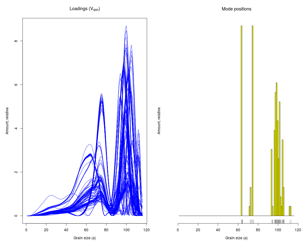
M1  <- test.robustness(X = X, q = q, l = l,
                       ol.rej = 1, mRt.rej = 0.8,
                       plot = TRUE,
                       colour = c(4, 7),
                       xlab = c(expression(paste("Grain size (", phi, ")",
                                                 sep = "")),
                                expression(paste("Grain size (", phi, ")",
                                                 sep = ""))))

## Example 2 -  perform the test without rejection criteria and plots
P  <- cbind(rep(q[1], length(l)),
            rep(q[3], length(l)),
            l)
M2  <- test.robustness(X = X, P = P)

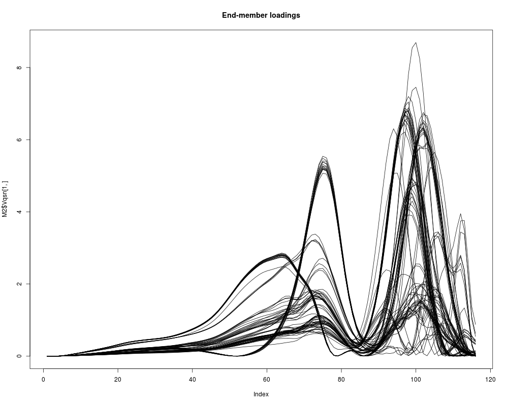
## Plot 1 - end-member loadings which do not overlap and yielded mRt > 0.80.
plot(M2$Vqsn[1,], type = "l", ylim = c(0, max(M2$Vqsn, na.rm = TRUE)),
     main = "End-member loadings")
  for (i in 2:nrow(M2$Vqsn)) lines(M2$Vqsn[i,])

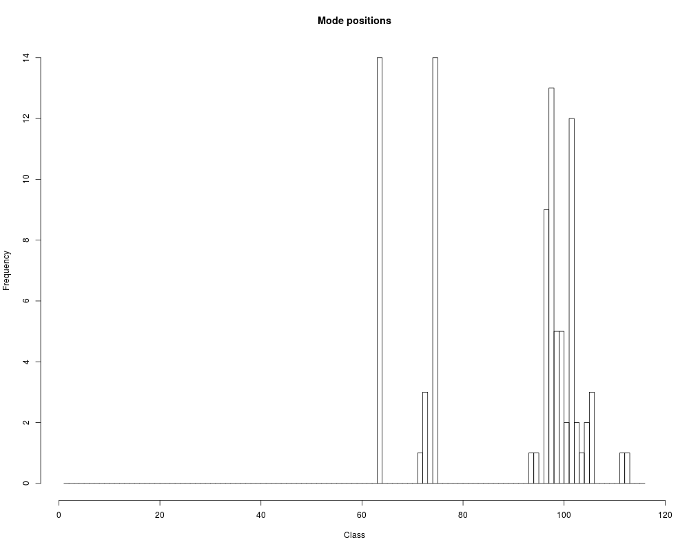
# Plot 2 - histogram of mode positions
hist(M2$modes,
     breaks = 1:ncol(X),
     main = "Mode positions",
     xlab = "Class")

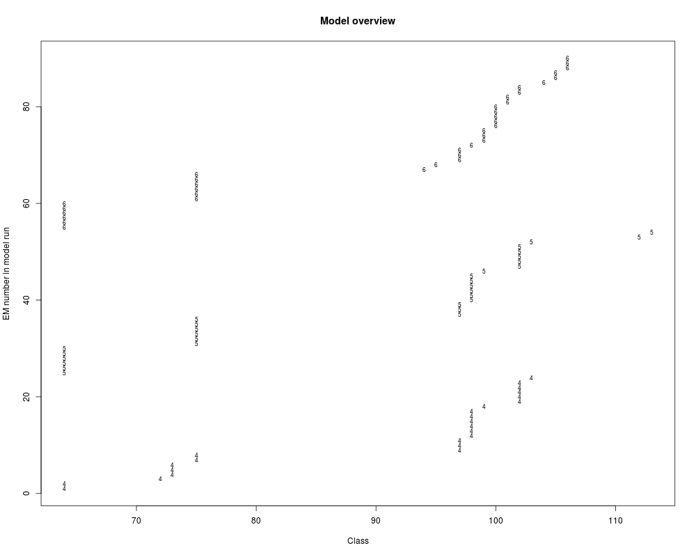
# Plot 3 - positions of modelled end-member modes by number of end-members
# Note how scatter in end-member position decreases for the "correct" number
# of modelled end-members (6) and an appropriate weight limit (ca. 0.1).
ii <- order(M2$q, M2$modes)
modes <- t(rbind(M2$modes, M2$q))[ii,]
plot(modes[,1],
     seq(1, nrow(modes)),
     main = "Model overview",
     xlab = "Class",
     ylab = "EM number in model run",
     pch = as.character(modes[,2]),
     cex = 0.7)

# Illustrate mode positions as stem-and-leave-plot, useful as a simple
# check, which mode maxima are consistently fall into which grain-size
# class (useful to define "limits" in robust.EM).
stem(M2$modes, scale = 2)

Results

R version 3.3.1 (2016-06-21) -- "Bug in Your Hair"
Copyright (C) 2016 The R Foundation for Statistical Computing
Platform: x86_64-pc-linux-gnu (64-bit)

R is free software and comes with ABSOLUTELY NO WARRANTY.
You are welcome to redistribute it under certain conditions.
Type 'license()' or 'licence()' for distribution details.

R is a collaborative project with many contributors.
Type 'contributors()' for more information and
'citation()' on how to cite R or R packages in publications.

Type 'demo()' for some demos, 'help()' for on-line help, or
'help.start()' for an HTML browser interface to help.
Type 'q()' to quit R.

> library(EMMAgeo)
Loading required package: GPArotation
Loading required package: limSolve
Loading required package: shape
Loading required package: shiny
> png(filename="/home/ddbj/snapshot/RGM3/R_CC/result/EMMAgeo/test.robustness.Rd_%03d_medium.png", width=480, height=480)
> ### Name: test.robustness
> ### Title: Function to test model robustness.
> ### Aliases: test.robustness
> ### Keywords: EMMA
> 
> ### ** Examples
> 
> ## load example data set
> data(X, envir = environment())
> 
> ## Example 1 - perform the most simple test
> q  <- 4:7
> l <- seq(from = 0, to = 0.1, by = 0.02)
> 
> M1  <- test.robustness(X = X, q = q, l = l,
+                        ol.rej = 1, mRt.rej = 0.8,
+                        plot = TRUE,
+                        colour = c(4, 7),
+                        xlab = c(expression(paste("Grain size (", phi, ")",
+                                                  sep = "")),
+                                 expression(paste("Grain size (", phi, ")",
+                                                  sep = ""))))
> 
> ## Example 2 -  perform the test without rejection criteria and plots
> P  <- cbind(rep(q[1], length(l)),
+             rep(q[3], length(l)),
+             l)
> M2  <- test.robustness(X = X, P = P)
> 
> ## Plot 1 - end-member loadings which do not overlap and yielded mRt > 0.80.
> plot(M2$Vqsn[1,], type = "l", ylim = c(0, max(M2$Vqsn, na.rm = TRUE)),
+      main = "End-member loadings")
>   for (i in 2:nrow(M2$Vqsn)) lines(M2$Vqsn[i,])
> 
> # Plot 2 - histogram of mode positions
> hist(M2$modes,
+      breaks = 1:ncol(X),
+      main = "Mode positions",
+      xlab = "Class")
> 
> # Plot 3 - positions of modelled end-member modes by number of end-members
> # Note how scatter in end-member position decreases for the "correct" number
> # of modelled end-members (6) and an appropriate weight limit (ca. 0.1).
> ii <- order(M2$q, M2$modes)
> modes <- t(rbind(M2$modes, M2$q))[ii,]
> plot(modes[,1],
+      seq(1, nrow(modes)),
+      main = "Model overview",
+      xlab = "Class",
+      ylab = "EM number in model run",
+      pch = as.character(modes[,2]),
+      cex = 0.7)
> 
> # Illustrate mode positions as stem-and-leave-plot, useful as a simple
> # check, which mode maxima are consistently fall into which grain-size
> # class (useful to define "limits" in robust.EM).
> stem(M2$modes, scale = 2)

  The decimal point is at the |

   64 | 00000000000000
   66 | 
   68 | 
   70 | 
   72 | 0000
   74 | 00000000000000
   76 | 
   78 | 
   80 | 
   82 | 
   84 | 
   86 | 
   88 | 
   90 | 
   92 | 
   94 | 00
   96 | 000000000
   98 | 000000000000000000
  100 | 0000000
  102 | 00000000000000
  104 | 000
  106 | 000
  108 | 
  110 | 
  112 | 00

> 
> 
> 
> 
> 
> dev.off()
null device 
          1 
>