R Graphical Manual

Browse All

Last data update: 2014.03.03

R: Bayesian, single arm, two endpoint trial designs, using loss...

bayes_binom_two_loss

R Documentation

Bayesian, single arm, two endpoint trial designs, using loss functions to make decisions

Description

Computes the decision rules for a single arm, two endpoint bayesian trial using a region of acceptable designs and loss functions to make decisions. This program assumes that the two endpoints are independent. A number of region spaces are provided. This function has the option of providing pre-existing decision matrices to skip this section if you wish to run additional simulations on an already computed design.

Usage

bayes_binom_two_loss(t, r, reviews, pra, prb, pta, ptb,
 l_alpha_beta, l_alpha_c, stage_after_trial, fun.integrate,
 efficacy_critical_value, toxicity_critical_value,
 futility_critical_value, no_toxicity_critical_value, decision=NULL,   
 W=NULL, fun.graph=NULL, ...)

Arguments

`t,r`	A vector of the probability of response and toxicity for the simulation scenarios used to compute frequentist properties. The print function requires the first to be the alternative hypothesis and subsequent entries to be the three null hypotheses. This can be run with any scenario when not using the print method
`reviews`	A vector of the number of patients each interim and final analysis will occur at
`pra,prb,pta,ptb`	Numeric values for the beta prior distribution to be used
`l_alpha_beta,l_alpha_c`	The two loss function variables weighting between stopping early for futility or efficacy and continuing the trial
`fun.integrate`	function used to integrate the probability of being in the region of interest given the posterior distributions of the data and prior information
`stage_after_trial`	Optional argument for censored stages after the trial has completed. This is likely to create a region of inclusiveness upon concluding the trial
`futility_critical_value, efficacy_critical_value, toxicity_critical_value, no_toxicity_critical_value`	Four values, for the critical values to be used as thresholds for the posterior distribution
`decision`	Optional input the decision matrices from a previous run to perform additional frequentist simulations on the design.
`W`	Optional input the posterior probabilities from a previous run to perform additional frequentist simulations on the design.
`fun.graph`	Optional function printing a graph of the region of interest. No region is plotted if this is left blank
`...`	Options passed to the integration function

Details

Returns an object of S4 class trialDesign_binom_two-class. This has plot and print methods. For comparison between designs saved as trialDesign_binom_two objects there is a print function for the S3 class list_trialDesign_binom_two.

The following region spaces are included in the package: tradeoff_square_integrate tradeoff_square_graph tradeoff_ratio_intercepts tradeoff_linear_graph tradeoff_ratio_integrate tradeoff_ratio_graph tradeoff_ellipse_integrate tradeoff_ellipse_graph

Value

Returns an object of class trialDesign_binom_two

References

Chen Y, Smith BJ. Adaptive group sequential design for phase II clinical trials: a Bayesian decision theoretic approach. Stat Med 2009; 28: 3347-3362.

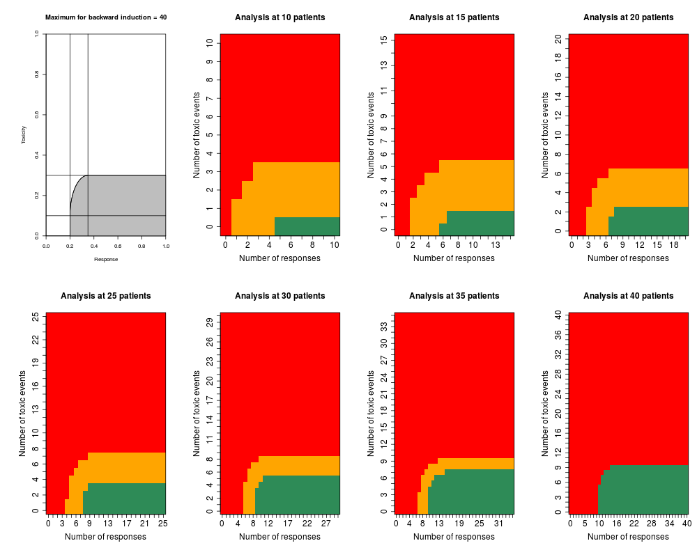
Examples

# modelled toxicity probability
t=c(0.1,0.1,0.3,0.3)
# modelled response probability
r=c(0.35,0.2,0.2,0.35)

reviews=c(10,15,20,25,30,35,40)
stage_after_trial=40

# uniform prior
pra=1;prb=1;pta=1;ptb=1

efficacy_critical_value=0.2
futility_critical_value=0.35
toxicity_critical_value=0.1
no_toxicity_critical_value=0.3

# alpha/beta ratio
l_alpha_beta=3
# cost of continuing compared to cost of alpha
l_alpha_c=750

efficacy_region_min=0.2
toxicity_region_max=0.3

########################################
# square region
s=bayes_binom_two_loss(t,r,reviews,pra,prb,pta,ptb,l_alpha_beta,
l_alpha_c,stage_after_trial,fun.integrate=tradeoff_square_integrate,
fun.graph=tradeoff_square_graph,efficacy_critical_value,
toxicity_critical_value,futility_critical_value,
no_toxicity_critical_value,efficacy_region_min=efficacy_region_min,
toxicity_region_max=toxicity_region_max)

plot(s)


########################################
# ellipse region
efficacy_region_min=0.2
efficacy_region_max=0.35
toxicity_region_min=0.1
toxicity_region_max=0.3


s=bayes_binom_two_loss(t,r,reviews,pra,prb,pta,ptb,l_alpha_beta,
l_alpha_c,stage_after_trial,fun.integrate=tradeoff_ellipse_integrate,
fun.graph=tradeoff_ellipse_graph,efficacy_critical_value,
toxicity_critical_value,futility_critical_value,
no_toxicity_critical_value,efficacy_region_min=efficacy_region_min,
toxicity_region_max=toxicity_region_max,
efficacy_region_max=efficacy_region_max,
toxicity_region_min=toxicity_region_min)


plot(s)

Results


R version 3.3.1 (2016-06-21) -- "Bug in Your Hair"
Copyright (C) 2016 The R Foundation for Statistical Computing
Platform: x86_64-pc-linux-gnu (64-bit)

R is free software and comes with ABSOLUTELY NO WARRANTY.
You are welcome to redistribute it under certain conditions.
Type 'license()' or 'licence()' for distribution details.

R is a collaborative project with many contributors.
Type 'contributors()' for more information and
'citation()' on how to cite R or R packages in publications.

Type 'demo()' for some demos, 'help()' for on-line help, or
'help.start()' for an HTML browser interface to help.
Type 'q()' to quit R.

> library(EurosarcBayes)
Loading required package: shiny
Loading required package: VGAM
Loading required package: stats4
Loading required package: splines
Loading required package: data.table
Loading required package: plyr
Loading required package: clinfun
> png(filename="/home/ddbj/snapshot/RGM3/R_CC/result/EurosarcBayes/bayes_binom_two_loss.Rd_%03d_medium.png", width=480, height=480)
> ### Name: bayes_binom_two_loss
> ### Title: Bayesian, single arm, two endpoint trial designs, using loss
> ###   functions to make decisions
> ### Aliases: bayes_binom_two_loss
> 
> ### ** Examples
> 
> # modelled toxicity probability
> t=c(0.1,0.1,0.3,0.3)
> # modelled response probability
> r=c(0.35,0.2,0.2,0.35)
> 
> reviews=c(10,15,20,25,30,35,40)
> stage_after_trial=40
> 
> # uniform prior
> pra=1;prb=1;pta=1;ptb=1
> 
> efficacy_critical_value=0.2
> futility_critical_value=0.35
> toxicity_critical_value=0.1
> no_toxicity_critical_value=0.3
> 
> # alpha/beta ratio
> l_alpha_beta=3
> # cost of continuing compared to cost of alpha
> l_alpha_c=750
> 
> efficacy_region_min=0.2
> toxicity_region_max=0.3
> 
> ########################################
> # square region
> s=bayes_binom_two_loss(t,r,reviews,pra,prb,pta,ptb,l_alpha_beta,
+ l_alpha_c,stage_after_trial,fun.integrate=tradeoff_square_integrate,
+ fun.graph=tradeoff_square_graph,efficacy_critical_value,
+ toxicity_critical_value,futility_critical_value,
+ no_toxicity_critical_value,efficacy_region_min=efficacy_region_min,
+ toxicity_region_max=toxicity_region_max)
[1] "The cost function is constant for all patients"
cut-points at each analysis
  patient review low toxicity high toxicity poor outcome good outcome
1             10            0             4            0            5
2             15            1             6            1            6
3             20            2             7            2            7
4             25            3             8            3            8
5             30            5             9            5            9
6             35            7            10            6           10
7             40            9            10            9           10

Frequentist properties of design
                                  Stopping rules T=0.1, R=0.35 T=0.1, R=0.2
1                 Stop early - Futility/Toxicity         10.72        58.54
4 Continue to final analysis - Futility/Toxicity          2.63        16.32
2                          Stop early - Efficacy         80.57        18.19
3          Continue to final analysis - Efficacy          6.08         6.95
6          Expected number of patients recruited         22.70        24.94
  T=0.3, R=0.2 T=0.3, R=0.35
1        93.02         77.56
4         2.60          6.73
2         2.99         11.10
3         1.39          4.61
6        15.56         20.04

Bayesian properties of trial design
  n T>0.3 T>0.1 T>0.3 T>0.1 R>0.2 R>0.35 R>0.2 R>0.35
 10 0.020 0.314 0.790 0.997 0.086  0.009 0.988  0.851
 15 0.026 0.515 0.825 0.999 0.141  0.010 0.973  0.688
 20 0.027 0.648 0.723 0.999 0.179  0.009 0.957  0.536
 25 0.026 0.741 0.627 0.999 0.207  0.007 0.941  0.411
 30 0.063 0.917 0.542 0.999 0.393  0.018 0.925  0.311
 35 0.112 0.976 0.466 0.999 0.401  0.013 0.911  0.234
 40 0.170 0.994 0.275 0.998 0.704  0.052 0.818  0.102

Futility     P(R<0.35)=0.948
Efficacy     P(R>0.2)=0.818

Toxicity ok  P(T<0.3)=0.83
Toxicity     P(T>0.1)=0.997> 
> plot(s)
> 
> 
> ########################################
> # ellipse region
> efficacy_region_min=0.2
> efficacy_region_max=0.35
> toxicity_region_min=0.1
> toxicity_region_max=0.3
> 
> 
> s=bayes_binom_two_loss(t,r,reviews,pra,prb,pta,ptb,l_alpha_beta,
+ l_alpha_c,stage_after_trial,fun.integrate=tradeoff_ellipse_integrate,
+ fun.graph=tradeoff_ellipse_graph,efficacy_critical_value,
+ toxicity_critical_value,futility_critical_value,
+ no_toxicity_critical_value,efficacy_region_min=efficacy_region_min,
+ toxicity_region_max=toxicity_region_max,
+ efficacy_region_max=efficacy_region_max,
+ toxicity_region_min=toxicity_region_min)
[1] "The cost function is constant for all patients"
cut-points at each analysis
  patient review low toxicity high toxicity poor outcome good outcome
1             10            0             4            0            5
2             15            1             6            1            6
3             20            2             7            2            7
4             25            3             8            3            8
5             30            5             9            5            9
6             35            7            10            6           10
7             40            9            10            9           10

Frequentist properties of design
                                  Stopping rules T=0.1, R=0.35 T=0.1, R=0.2
1                 Stop early - Futility/Toxicity         13.09        62.94
4 Continue to final analysis - Futility/Toxicity          3.34        13.69
2                          Stop early - Efficacy         76.07        16.57
3          Continue to final analysis - Efficacy          7.51         6.81
6          Expected number of patients recruited         23.64        24.64
  T=0.3, R=0.2 T=0.3, R=0.35
1        94.91         80.72
4         2.21          5.63
2         1.86          9.27
3         1.02          4.37
6        14.77         19.29

Bayesian properties of trial design
  n T>0.3 T>0.1 T>0.3 T>0.1 R>0.2 R>0.35 R>0.2 R>0.35
 10 0.020 0.314 0.790 0.997 0.086  0.009 0.988  0.851
 15 0.026 0.515 0.825 0.999 0.141  0.010 0.973  0.688
 20 0.027 0.648 0.723 0.999 0.179  0.009 0.957  0.536
 25 0.026 0.741 0.627 0.999 0.207  0.007 0.941  0.411
 30 0.063 0.917 0.542 0.999 0.393  0.018 0.925  0.311
 35 0.112 0.976 0.466 0.999 0.401  0.013 0.911  0.234
 40 0.170 0.994 0.275 0.998 0.704  0.052 0.818  0.102

Futility     P(R<0.35)=0.948
Efficacy     P(R>0.2)=0.818

Toxicity ok  P(T<0.3)=0.83
Toxicity     P(T>0.1)=0.997> 
> 
> plot(s)
> 
> 
> 
> 
> 
> 
> dev.off()
null device 
          1 
>