Bayesian, single arm, two endpoint trial designs.

Description

Computes the decision rules for a single arm, two endpoint bayesian trial using the likelihood of success to make decisions. This program assumes that the two endpoints are independent.

Usage

bayes_binom_two_postlike(t, r, reviews, pra, prb, pta, ptb,
 efficacy_critical_value, efficacy_prob_stop, toxicity_critical_value,
 toxicity_prob_stop, int_combined_prob, int_futility_prob,
 int_toxicity_prob, int_efficacy_prob, futility_critical_value,
 no_toxicity_critical_value)

Arguments

Details

Returns an object of S4 class trialDesign_binom_two-class. This has plot and print methods. For comparison between designs saved as trialDesign_binom_two objects there is a print function for the S3 class list_trialDesign_binom_two.

Value

Returns an object of class trialDesign_binom_two

See Also

bayes_binom_two_postprob, bayes_binom_two_postlike,bayes_binom_two_loss

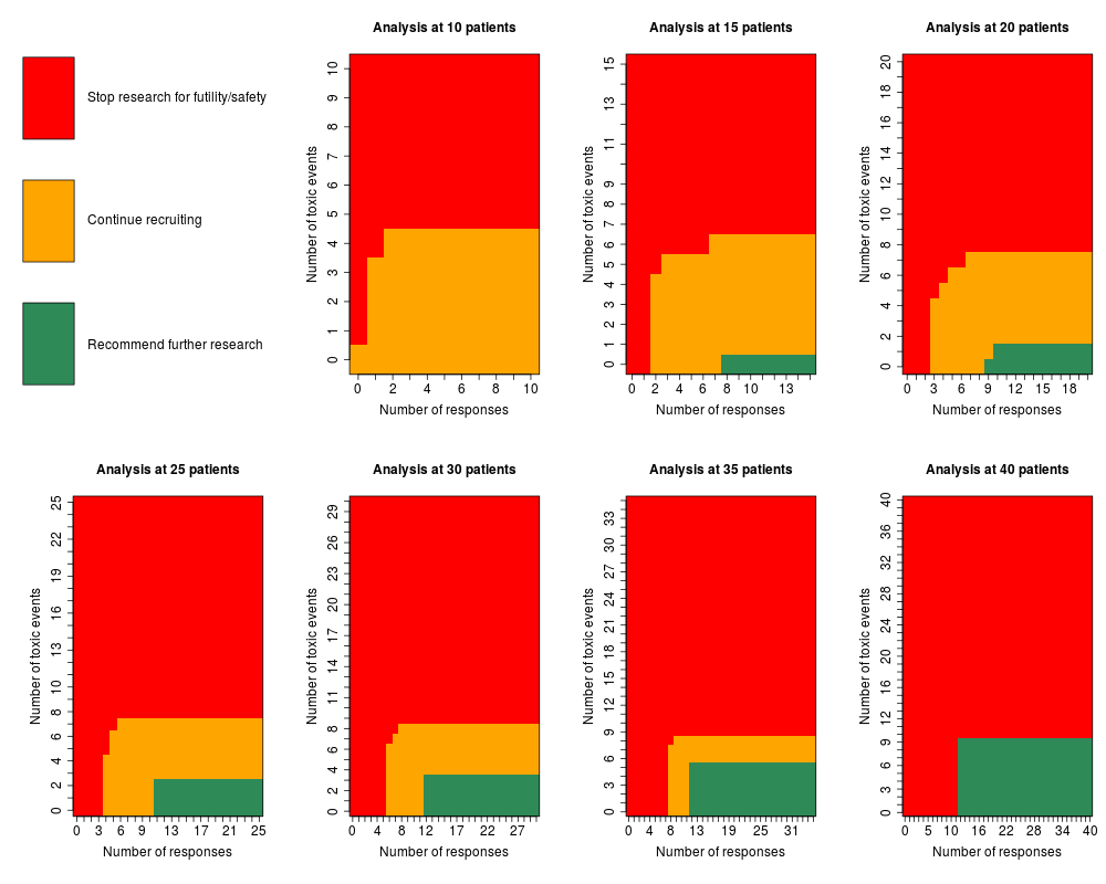
Examples

# modelled toxicity probability
t=c(0.1,0.1,0.3,0.3)
# modelled response probability
r=c(0.35,0.2,0.2,0.35)

reviews=c(10,15,20,25,30,35,40)

# uniform prior
pra=1;prb=1;pta=1;ptb=1

# End of trial stopping rules for success
efficacy_critical_value=0.2
efficacy_prob_stop=0.9
toxicity_critical_value=0.2
toxicity_prob_stop=0.8

# interim required probability to stop
int_combined_prob=0.99
int_futility_prob=1
int_toxicity_prob=1
int_efficacy_prob=0.99

# unused in the design for comparison to previous design
futility_critical_value=0.35
no_toxicity_critical_value=0.3

s=bayes_binom_two_postlike(t,r,reviews,pra,prb,pta,ptb,
efficacy_critical_value,efficacy_prob_stop,toxicity_critical_value,
toxicity_prob_stop,int_combined_prob,int_futility_prob,
int_toxicity_prob,int_efficacy_prob,futility_critical_value,
no_toxicity_critical_value)

s

plot(s)

Results

R version 3.3.1 (2016-06-21) -- "Bug in Your Hair"
Copyright (C) 2016 The R Foundation for Statistical Computing
Platform: x86_64-pc-linux-gnu (64-bit)

R is free software and comes with ABSOLUTELY NO WARRANTY.
You are welcome to redistribute it under certain conditions.
Type 'license()' or 'licence()' for distribution details.

R is a collaborative project with many contributors.
Type 'contributors()' for more information and
'citation()' on how to cite R or R packages in publications.

Type 'demo()' for some demos, 'help()' for on-line help, or
'help.start()' for an HTML browser interface to help.
Type 'q()' to quit R.

> library(EurosarcBayes)
Loading required package: shiny
Loading required package: VGAM
Loading required package: stats4
Loading required package: splines
Loading required package: data.table
Loading required package: plyr
Loading required package: clinfun
> png(filename="/home/ddbj/snapshot/RGM3/R_CC/result/EurosarcBayes/bayes_binom_two_postlike.Rd_%03d_medium.png", width=480, height=480)
> ### Name: bayes_binom_two_postlike
> ### Title: Bayesian, single arm, two endpoint trial designs.
> ### Aliases: bayes_binom_two_postlike
> 
> ### ** Examples
> 
> # modelled toxicity probability
> t=c(0.1,0.1,0.3,0.3)
> # modelled response probability
> r=c(0.35,0.2,0.2,0.35)
> 
> reviews=c(10,15,20,25,30,35,40)
> 
> # uniform prior
> pra=1;prb=1;pta=1;ptb=1
> 
> # End of trial stopping rules for success
> efficacy_critical_value=0.2
> efficacy_prob_stop=0.9
> toxicity_critical_value=0.2
> toxicity_prob_stop=0.8
> 
> # interim required probability to stop
> int_combined_prob=0.99
> int_futility_prob=1
> int_toxicity_prob=1
> int_efficacy_prob=0.99
> 
> # unused in the design for comparison to previous design
> futility_critical_value=0.35
> no_toxicity_critical_value=0.3
> 
> s=bayes_binom_two_postlike(t,r,reviews,pra,prb,pta,ptb,
+ efficacy_critical_value,efficacy_prob_stop,toxicity_critical_value,
+ toxicity_prob_stop,int_combined_prob,int_futility_prob,
+ int_toxicity_prob,int_efficacy_prob,futility_critical_value,
+ no_toxicity_critical_value)
cut-points at each analysis
  patient review low toxicity high toxicity poor outcome good outcome
1             10           NA             5           NA           NA
2             15            0             7            1            8
3             20            1             8            2            9
4             25            2             8            3           11
5             30            3             9            5           12
6             35            5             9            7           12
7             40            9            10           11           12

Frequentist properties of design
                                  Stopping rules T=0.1, R=0.35 T=0.1, R=0.2
1                 Stop early - Futility/Toxicity          7.11        63.61
4 Continue to final analysis - Futility/Toxicity         14.82        27.83
2                          Stop early - Efficacy         54.16         3.25
3          Continue to final analysis - Efficacy         23.90         5.32
6          Expected number of patients recruited         33.51        29.81
  T=0.3, R=0.2 T=0.3, R=0.35
1        91.38         79.37
4         6.36          6.60
2         0.22          2.15
3         2.04         11.88
6        20.30         25.46

Bayesian properties of trial design
  n T>0.3 T>0.2 T>0.3 T>0.2 R>0.2 R>0.35 R>0.2 R>0.35
 10    NA    NA 0.922 0.988    NA     NA    NA     NA
 15 0.003 0.028 0.926 0.993 0.141  0.010 0.999  0.933
 20 0.006 0.058 0.852 0.986 0.179  0.009 0.996  0.838
 25 0.007 0.084 0.627 0.941 0.207  0.007 0.998  0.838
 30 0.007 0.107 0.542 0.925 0.393  0.018 0.996  0.736
 35 0.022 0.246 0.325 0.832 0.566  0.033 0.982  0.493
 40 0.170 0.704 0.275 0.818 0.898  0.176 0.948  0.276

Futility     P(R<0.35)=0.824
Efficacy     P(R>0.2)=0.948

Toxicity ok  P(T<0.3)=0.83
Toxicity     P(T>0.2)=0.818> 
> s
                    n  alpha   beta Exp.P0 Exp.P1 post.futility post.efficacy
 10,15,20,25,30,35,40 0.1403 0.2194  29.81  33.51         0.824         0.948
 post.toxicity post.no_toxicity
         0.818             0.83
> 
> plot(s)
> 
> 
> 
> 
> 
> dev.off()
null device 
          1 
>