Functions for integration for Bayesian loss methodology

Description

An integral and graph for an acceptable region for the bayesian loss function approach (see bayes_binom_two_loss)

Usage

tradeoff_linear_integrate(ar, br, at, bt, efficacy_region_min, 
	toxicity_region_max, efficacy_region_max, toxicity_region_min)

tradeoff_linear_graph(input)

Arguments

Value

Returns value of the integration.

References

Chen Y, Smith BJ. Adaptive group sequential design for phase II clinical trials: a Bayesian decision theoretic approach. Stat Med 2009; 28: 3347-3362.

See Also

bayes_binom_two_loss

Integration functions and corresponding graphs: tradeoff_square_integrate,tradeoff_ellipse_integrate,tradeoff_linear_integrate,tradeoff_ratio_integrate

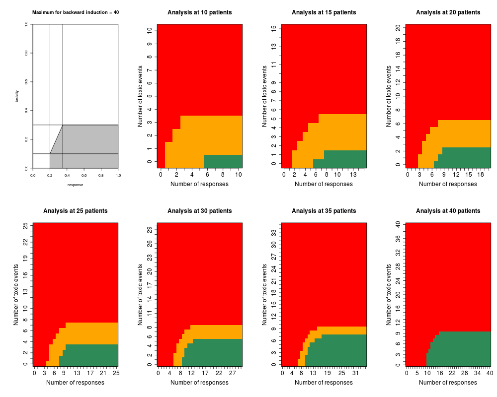
Examples

# modelled toxicity probability
t=c(0.1,0.1,0.3,0.3)
# modelled response probability
r=c(0.35,0.2,0.2,0.35)

reviews=c(10,15,20,25,30,35,40)
stage_after_trial=40

# uniform prior
pra=1;prb=1;pta=1;ptb=1

efficacy_critical_value=0.2
futility_critical_value=0.35
toxicity_critical_value=0.1
no_toxicity_critical_value=0.3

# alpha/beta ratio
l_alpha_beta=3
# cost of continuing compared to cost of alpha
l_alpha_c=750

efficacy_region_min=0.2
toxicity_region_max=0.3

########################################
# linear region
efficacy_region_min=0.2
efficacy_region_max=0.35
toxicity_region_min=0.1
toxicity_region_max=0.3

s=bayes_binom_two_loss(t,r,reviews,pra,prb,pta,ptb,l_alpha_beta,
	l_alpha_c,stage_after_trial,fun.integrate=tradeoff_linear_integrate,
	fun.graph=tradeoff_linear_graph,efficacy_critical_value,
	toxicity_critical_value,futility_critical_value,
	no_toxicity_critical_value,efficacy_region_min=efficacy_region_min,
	toxicity_region_max=toxicity_region_max,
	efficacy_region_max=efficacy_region_max,
	toxicity_region_min=toxicity_region_min)

plot(s)

Results

R version 3.3.1 (2016-06-21) -- "Bug in Your Hair"
Copyright (C) 2016 The R Foundation for Statistical Computing
Platform: x86_64-pc-linux-gnu (64-bit)

R is free software and comes with ABSOLUTELY NO WARRANTY.
You are welcome to redistribute it under certain conditions.
Type 'license()' or 'licence()' for distribution details.

R is a collaborative project with many contributors.
Type 'contributors()' for more information and
'citation()' on how to cite R or R packages in publications.

Type 'demo()' for some demos, 'help()' for on-line help, or
'help.start()' for an HTML browser interface to help.
Type 'q()' to quit R.

> library(EurosarcBayes)
Loading required package: shiny
Loading required package: VGAM
Loading required package: stats4
Loading required package: splines
Loading required package: data.table
Loading required package: plyr
Loading required package: clinfun
> png(filename="/home/ddbj/snapshot/RGM3/R_CC/result/EurosarcBayes/tradeoff_linear.Rd_%03d_medium.png", width=480, height=480)
> ### Name: tradeoff linear
> ### Title: Functions for integration for Bayesian loss methodology
> ### Aliases: tradeoff_linear_integrate tradeoff_linear_graph
> 
> ### ** Examples
> 
> # modelled toxicity probability
> t=c(0.1,0.1,0.3,0.3)
> # modelled response probability
> r=c(0.35,0.2,0.2,0.35)
> 
> reviews=c(10,15,20,25,30,35,40)
> stage_after_trial=40
> 
> # uniform prior
> pra=1;prb=1;pta=1;ptb=1
> 
> efficacy_critical_value=0.2
> futility_critical_value=0.35
> toxicity_critical_value=0.1
> no_toxicity_critical_value=0.3
> 
> # alpha/beta ratio
> l_alpha_beta=3
> # cost of continuing compared to cost of alpha
> l_alpha_c=750
> 
> efficacy_region_min=0.2
> toxicity_region_max=0.3
> 
> ########################################
> # linear region
> efficacy_region_min=0.2
> efficacy_region_max=0.35
> toxicity_region_min=0.1
> toxicity_region_max=0.3
> 
> s=bayes_binom_two_loss(t,r,reviews,pra,prb,pta,ptb,l_alpha_beta,
+ 	l_alpha_c,stage_after_trial,fun.integrate=tradeoff_linear_integrate,
+ 	fun.graph=tradeoff_linear_graph,efficacy_critical_value,
+ 	toxicity_critical_value,futility_critical_value,
+ 	no_toxicity_critical_value,efficacy_region_min=efficacy_region_min,
+ 	toxicity_region_max=toxicity_region_max,
+ 	efficacy_region_max=efficacy_region_max,
+ 	toxicity_region_min=toxicity_region_min)
[1] "The cost function is constant for all patients"
cut-points at each analysis
  patient review low toxicity high toxicity poor outcome good outcome
1             10            0             4            0            6
2             15            1             6            1            6
3             20            2             7            2            7
4             25            3             8            3            8
5             30            5             9            5            9
6             35            7            10            6           10
7             40            9            10            9           10

Frequentist properties of design
                                  Stopping rules T=0.1, R=0.35 T=0.1, R=0.2
1                 Stop early - Futility/Toxicity         20.40        73.02
4 Continue to final analysis - Futility/Toxicity          4.47         8.53
2                          Stop early - Efficacy         67.90        12.71
3          Continue to final analysis - Efficacy          7.22         5.74
6          Expected number of patients recruited         24.91        23.31
  T=0.3, R=0.2 T=0.3, R=0.35
1        97.55         85.59
4         1.03          4.18
2         1.00          6.75
3         0.42          3.48
6        13.80         18.33

Bayesian properties of trial design
  n T>0.3 T>0.1 T>0.3 T>0.1 R>0.2 R>0.35 R>0.2 R>0.35
 10 0.020 0.314 0.790 0.997 0.086  0.009 0.998  0.950
 15 0.026 0.515 0.825 0.999 0.141  0.010 0.973  0.688
 20 0.027 0.648 0.723 0.999 0.179  0.009 0.957  0.536
 25 0.026 0.741 0.627 0.999 0.207  0.007 0.941  0.411
 30 0.063 0.917 0.542 0.999 0.393  0.018 0.925  0.311
 35 0.112 0.976 0.466 0.999 0.401  0.013 0.911  0.234
 40 0.170 0.994 0.275 0.998 0.704  0.052 0.818  0.102

Futility     P(R<0.35)=0.948
Efficacy     P(R>0.2)=0.818

Toxicity ok  P(T<0.3)=0.83
Toxicity     P(T>0.1)=0.997> 
> plot(s)
> 
> 
> 
> 
> 
> 
> 
> dev.off()
null device 
          1 
>