Supported by Dr. Osamu Ogasawara and  . . |
|
Last data update: 2014.03.03 |
simulate Euclidean distances for sister pair data under 10 evolutionary modelsDescriptionsimulate Euclidean distances for sister pair data under 10 evolutionary models Usagesim.sisters(TIME, GRAD, GRAD2 = "NULL", parameters, model, MULT=1) Arguments
DetailsThis function is called by bootstrap.sister, but can also be used for customized routines to explore model power and to visualize what data is expected to look like under different evolutionary rates. ValueReturns a matrix with 3 columns corresponding to GRAD, TIME and simulated DIST. Author(s)Jason T. Weir ReferencesWeir JT, D Wheatcroft, & T Price. 2012. The role of ecological constraint in driving the evolution of avian song frequency across a latitudinal gradient. Evolution 66, 2773-2783. Weir JT, & D Wheatcroft. 2011. A latitudinal gradient in rates of evolution of avian syllable diversity and song length. Proceedings of the Royal Society of London, B 278, 1713-1720. See AlsosisterContinuous, bootstrap.sister Examples
##Example 1
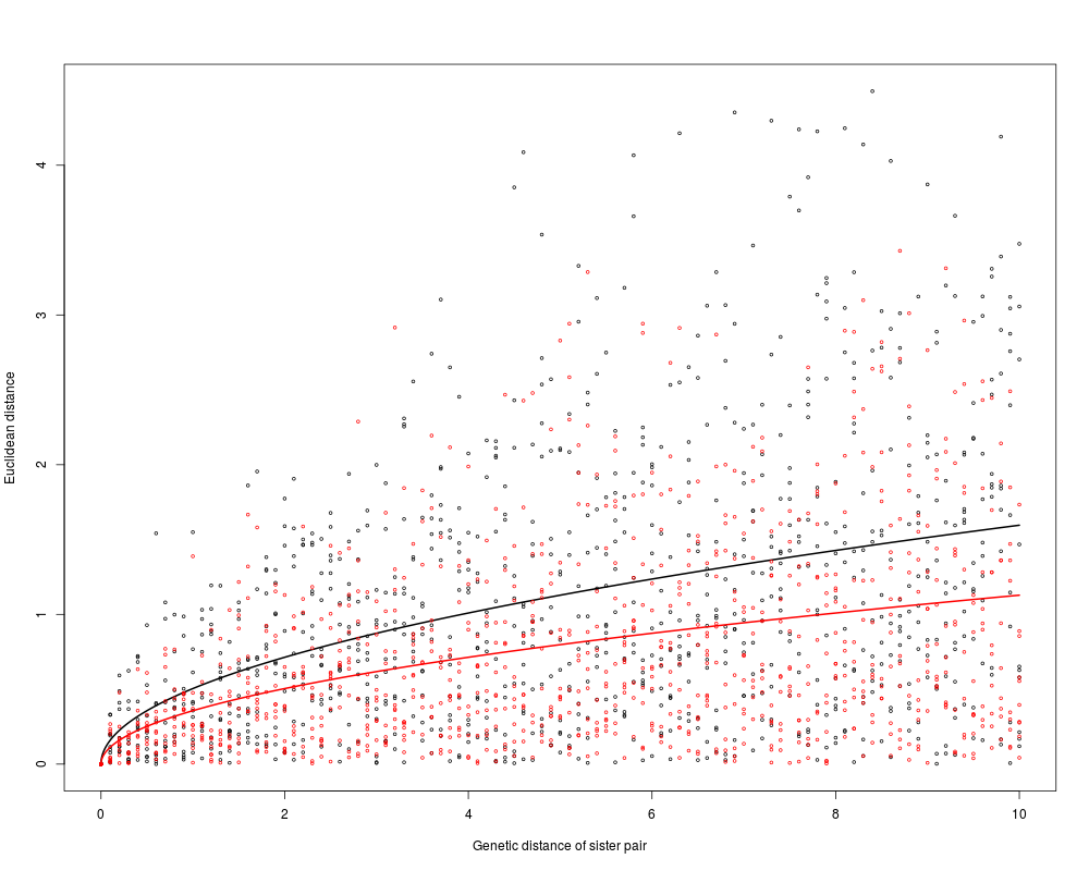
###This example graphically compares the distributions of simulated Euclidean
###distances under BM_null when Beta (evolutionary rate) is 0.1 and 0.2
TIME = c(0:100) * 0.1
GRAD = (0:100)*0 #BM_null does not require GRAD, thus simply make a dummy set of GRAD
DATA1 <- sim.sisters(TIME=TIME, GRAD=GRAD, parameters = c(0.2),
model=c("BM_null"), MULT=10)
DATA2 <- sim.sisters(TIME=TIME, GRAD=GRAD, parameters = c(0.1),
model=c("BM_null"), MULT=10)
plot(DATA1[,3] ~ DATA1[,2], xlab="Genetic distance of sister pair",
ylab = "Euclidean distance", cex=0.5)
expectation1 <- expectation.time(Beta = 0.2, Alpha="NULL", time.span=c(0, 10),
values="TRUE", plot=FALSE, quantile=FALSE)
lines(expectation1[,2] ~ expectation1[,1], lwd=2)
points(DATA2[,3] ~ DATA2[,2], col="red", cex=0.5)
expectation2 <- expectation.time(Beta = 0.1, Alpha="NULL", time.span=c(0, 10),
values="TRUE", plot=FALSE, quantile=FALSE)
lines(expectation2[,2] ~ expectation2[,1],col="red", lwd=2)
###Notice that doubling Beta still results in largely overlapping distributions
###of DIST at any given TIME, and the expectation (shown by lines) is not doubled.
##Example 2
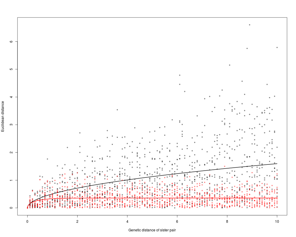
###graphically compare data simulated with the same evolutionary rate (Beta)
###under BM_null versus OU_null to see the effect of constraint (Alpha)
TIME = c(0:100) * 0.1
GRAD = (0:100)*0 #GRAD is not required by these models, so a dummy set of GRAD are provided
DATA1 <- sim.sisters(TIME=TIME, GRAD=GRAD, parameters = c(0.2),
model=c("BM_null"), MULT=10)
DATA2 <- sim.sisters(TIME=TIME, GRAD=GRAD, parameters = c(0.2, 1),
model=c("OU_null"), MULT=10)
plot(DATA1[,3] ~ DATA1[,2], xlab="Genetic distance of sister pair",
ylab = "Euclidean distance", cex=0.5)
expectation1 <- expectation.time(Beta = 0.2, Alpha="NULL", time.span=c(0, 10),
values="TRUE", plot=FALSE, quantile=FALSE)
lines(expectation1[,2] ~ expectation1[,1], lwd=2)
points(DATA2[,3] ~ DATA2[,2], col="red", cex=0.5)
expectation2 <- expectation.time(Beta = 0.2, Alpha=1, time.span=c(0, 10),
values="TRUE", plot=FALSE, quantile=FALSE)
lines(expectation2[,2] ~ expectation2[,1],col="red", lwd=2)
###Notice that DIST increases in a similar fashion under BM and OU until about
###TIME = 0.5 after which point the strong constraint in OU becomesevident.
Results
R version 3.3.1 (2016-06-21) -- "Bug in Your Hair"
Copyright (C) 2016 The R Foundation for Statistical Computing
Platform: x86_64-pc-linux-gnu (64-bit)

R is free software and comes with ABSOLUTELY NO WARRANTY.
You are welcome to redistribute it under certain conditions.
Type 'license()' or 'licence()' for distribution details.

R is a collaborative project with many contributors.
Type 'contributors()' for more information and
'citation()' on how to cite R or R packages in publications.

Type 'demo()' for some demos, 'help()' for on-line help, or
'help.start()' for an HTML browser interface to help.
Type 'q()' to quit R.

> library(EvoRAG)
> png(filename="/home/ddbj/snapshot/RGM3/R_CC/result/EvoRAG/sim.sisters.Rd_%03d_medium.png", width=480, height=480)
> ### Name: sim.sisters
> ### Title: simulate Euclidean distances for sister pair data under 10
> ###   evolutionary models
> ### Aliases: sim.sisters
> ### Keywords: Brownian Motion Ornstein Uhlenbeck Simulation
>
> ### ** Examples
>
> ##Example 1
>   ###This example graphically compares the distributions of simulated Euclidean
>   ###distances under BM_null when Beta (evolutionary rate) is 0.1 and 0.2
>   TIME = c(0:100) * 0.1
>   GRAD = (0:100)*0 #BM_null does not require GRAD, thus simply make a dummy set of GRAD
>   DATA1 <- sim.sisters(TIME=TIME, GRAD=GRAD, parameters = c(0.2),
+      model=c("BM_null"), MULT=10)
>   DATA2 <- sim.sisters(TIME=TIME, GRAD=GRAD, parameters = c(0.1),
+      model=c("BM_null"), MULT=10)
>   plot(DATA1[,3] ~ DATA1[,2], xlab="Genetic distance of sister pair",
+      ylab = "Euclidean distance", cex=0.5)
>   expectation1 <- expectation.time(Beta = 0.2, Alpha="NULL", time.span=c(0, 10),
+      values="TRUE", plot=FALSE, quantile=FALSE)
>   lines(expectation1[,2] ~ expectation1[,1], lwd=2)
>   points(DATA2[,3] ~ DATA2[,2], col="red",  cex=0.5)
>   expectation2 <- expectation.time(Beta = 0.1, Alpha="NULL", time.span=c(0, 10),
+       values="TRUE", plot=FALSE, quantile=FALSE)
>   lines(expectation2[,2] ~ expectation2[,1],col="red", lwd=2)
>   ###Notice that doubling Beta still results in largely overlapping distributions
>   ###of DIST at any given TIME, and the expectation (shown by lines) is not doubled.
>
> ##Example 2
>   ###graphically compare data simulated with the same evolutionary rate (Beta)
>   ###under BM_null versus OU_null to see the effect of constraint (Alpha)
>   TIME = c(0:100) * 0.1
>   GRAD = (0:100)*0 #GRAD is not required by these models, so a dummy set of GRAD are provided
>   DATA1 <- sim.sisters(TIME=TIME, GRAD=GRAD, parameters = c(0.2),
+      model=c("BM_null"), MULT=10)
>   DATA2 <- sim.sisters(TIME=TIME, GRAD=GRAD, parameters = c(0.2, 1),
+      model=c("OU_null"), MULT=10)
>   plot(DATA1[,3] ~ DATA1[,2], xlab="Genetic distance of sister pair",
+      ylab = "Euclidean distance", cex=0.5)
>   expectation1 <- expectation.time(Beta = 0.2, Alpha="NULL", time.span=c(0, 10),
+      values="TRUE", plot=FALSE, quantile=FALSE)
>   lines(expectation1[,2] ~ expectation1[,1], lwd=2)
>   points(DATA2[,3] ~ DATA2[,2], col="red", cex=0.5)
>   expectation2 <- expectation.time(Beta = 0.2, Alpha=1, time.span=c(0, 10),
+      values="TRUE", plot=FALSE, quantile=FALSE)
>   lines(expectation2[,2] ~ expectation2[,1],col="red", lwd=2)
>   ###Notice that DIST increases in a similar fashion under BM and OU until about
>   ###TIME = 0.5 after which point the strong constraint in OU becomesevident.
>
>
>
>
>
> dev.off()
null device
          1
>
|