Unconditional exact tests for 2x2 tables

Description

Calculates Barnard's or Boschloo's unconditional exact test for binomial or multinomial models

Usage

exact.test(data, alternative = "two.sided", npNumbers = 100, beta = 0.001,
           interval = FALSE, method = "Z-pooled", model = "Binomial", 
           cond.row = TRUE, to.plot = TRUE, ref.pvalue=TRUE)

Arguments

Details

Unconditional exact tests can be used for binomial or multinomial models. The binomial model assumes the row or column margins (but not both) are known in advance, while the multinomial model assumes only the total sample size is known beforehand. Conditional tests have both row and column margins fixed. The null hypothesis is that the rows and columns are independent. Under the binomial model, the user will need to input which margin is fixed (default is rows). vspace{3 mm}

Let X denote a generic 2x2 table with fixed sample sizes n_1 and n_2, X_0 denote the observed table, and T(X) represent the test statistic function. The null hypothesis can be written as p_1=p_2 equiv p. The p-value function with rows fixed is the product of two independent binomials:

P(X|p)= sup_{0 ≤q p ≤q 1} ∑_{T(X) ≥q T(X_0)} {n_1 choose x_{11}} {n_2 choose x_{21}} p^{x_{11}+x_{21}} (1-p)^{x_{12}+x_{13}}

The multinomial model is similar except the summand has a multinomial distribution with two nuisance parameters. vspace{3 mm}

There are several possible test statistics to determine the 'as or more extreme' tables seen in the index of summation. The method variable lets the user choose the test statistic being used. A brief description for each test statistic is given below (see References for more details): vspace{3 mm}

Let hat{p_1}=x_{11}/n_1, hat{p_2}=x_{21}/n_2, and hat{p}=(x_{11}+x_{21})/(n_1+n_2). vspace{3 mm}

Z-unpooled (or Wald):

Z_u(x_{11},x_{21})=frac{hat{p_2}-hat{p_1}}{√{frac{hat{p_1}(1-hat{p_1})}{n_1}+frac{hat{p_2}(1-hat{p_2})}{n_2}}}

Z-pooled (or Score):

Z_p(x_{11},x_{21})=frac{hat{p_2}-hat{p_1}}{√{frac{hat{p}(1-hat{p})}{n_1}+frac{hat{p}(1-hat{p})}{n_2}}}

Santner and Snell:

D(x_{11},x_{21})=hat{p_2}-hat{p_1}

Boschloo:

Uses the p-value from Fisher's exact test as the test statistic. vspace{3 mm}

CSM:

Starts with the most extreme table and adds other 'as or more extreme' tables one step at a time by maximizing the summand of the p-value function. This approach can be computationally intensive. vspace{0 mm}

CSM modified:

Starts with all tables that must be more extreme and adds other 'as or more extreme' tables one step at a time by maximizing the summand of the p-value function. This approach can be computationally intensive. vspace{3 mm}

CSM approximate:

Maximizes the summand of the p-value function for each possible table. Thus, the test statistic is the p-value function without the summation. This approach is less computationally intensive than the CSM test because the maximization is not repeated at each step. vspace{3 mm}

The supremum of the common success probability is taken over all values between 0 and 1. Another approach, proposed by Berger and Boos, is to take the supremum over a Clopper-Pearson confidence interval. This approach adds a small penalty to the p-value to ensure a level-α test, but eliminates unlikely probabilities from inflating the p-value. The p-value function becomes:

P(X|p)= ≤ft(sup_{p in C_β} ∑_{T(X) ≥q T(X_0)} {n_1 choose x_{11}} {n_2 choose x_{21}} p^{x_{11}+x_{21}} (1-p)^{x_{12}+x_{13}} ight) + β

where C_β is the 100(1-β)% confidence interval of p vspace{3 mm}

There are many ways to define the two-sided p-value; this code uses the fisher.test() approach by summing the probabilities for both sides of the table.

Value

Warning

Multinomial models and CSM tests may take a very long time, even for sample sizes less than 100.

Note

See formulas in link: http://cran.r-project.org/web/packages/Exact/Exact.pdf. CSM test and multinomial models are much more computationally intensive. I have also spent a greater amount of time making the computations for the binomial models more efficient; future work will be devoted to improving the multinomial models. Boschloo's test also takes longer due to calculating Fisher's p-value for every possible table; however, a created function that calculates Fisher's test efficiently is utilized. Increasing the number of nuisance parameters considered and refining the p-value will increase the computation time.

Author(s)

Peter Calhoun

References

This code was influenced by the FORTRAN program located at http://www4.stat.ncsu.edu/~boos/exact/

See Also

fisher.test, Barnard, and exact2x2

Examples

data<-matrix(c(7,8,12,3),2,2,byrow=TRUE)
exact.test(data,alternative="less",to.plot=TRUE)
exact.test(data,alternative="two.sided",interval=TRUE,beta=0.001,npNumbers=100,method="Z-pooled",
           to.plot=FALSE)
exact.test(data,alternative="two.sided",interval=TRUE,beta=0.001,npNumbers=100,method="Boschloo",
           to.plot=FALSE)

#Example from Barnard's (1947) appendix:
data<-matrix(c(4,0,3,7),2,2,dimnames=list(c("Box 1","Box 2"),c("Defective","Not Defective")))
exact.test(data,method="CSM",alternative="two.sided")

data<-matrix(c(6,8,4,3),2,2,byrow=TRUE)
exact.test(data,model="Multinomial",alternative="less",method="Z-pooled")

Results

R version 3.3.1 (2016-06-21) -- "Bug in Your Hair"
Copyright (C) 2016 The R Foundation for Statistical Computing
Platform: x86_64-pc-linux-gnu (64-bit)

R is free software and comes with ABSOLUTELY NO WARRANTY.
You are welcome to redistribute it under certain conditions.
Type 'license()' or 'licence()' for distribution details.

R is a collaborative project with many contributors.
Type 'contributors()' for more information and
'citation()' on how to cite R or R packages in publications.

Type 'demo()' for some demos, 'help()' for on-line help, or
'help.start()' for an HTML browser interface to help.
Type 'q()' to quit R.

> library(Exact)
> png(filename="/home/ddbj/snapshot/RGM3/R_CC/result/Exact/exact.test.Rd_%03d_medium.png", width=480, height=480)
> ### Name: exact.test
> ### Title: Unconditional exact tests for 2x2 tables
> ### Aliases: exact.test
> ### Keywords: Barnard Boschloo Unconditional Exact Nonparametric
> 
> ### ** Examples
> 
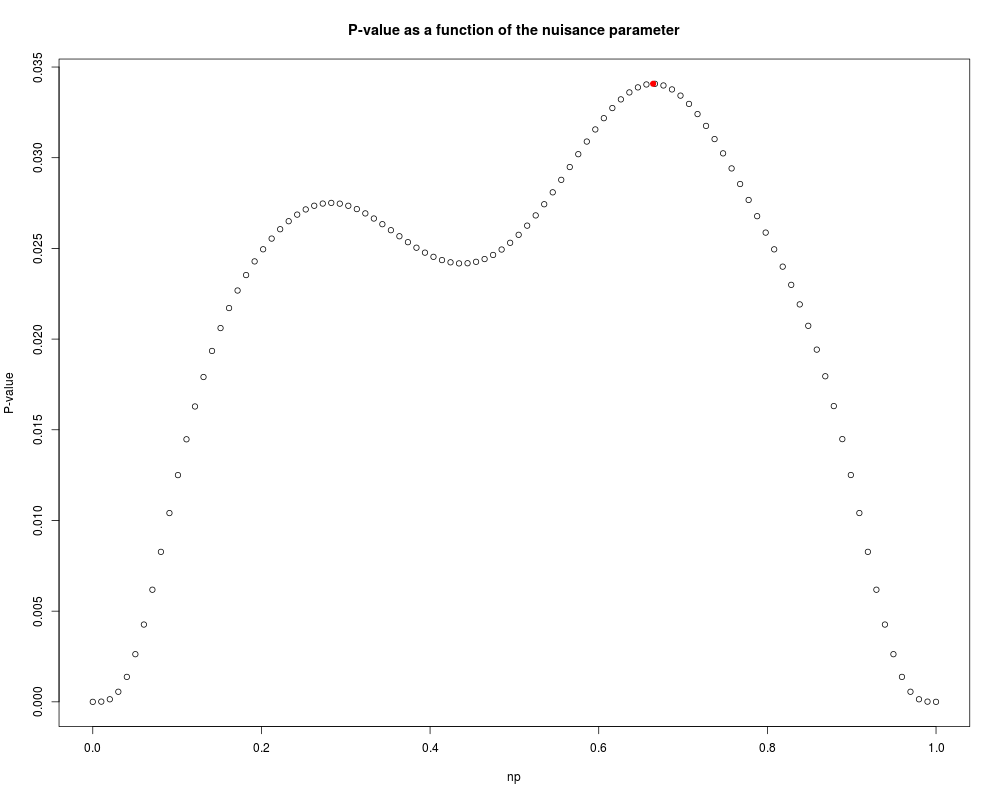
> data<-matrix(c(7,8,12,3),2,2,byrow=TRUE)
> exact.test(data,alternative="less",to.plot=TRUE)
$model
[1] "Binomial"

$method
[1] "Z-pooled"

$alternative
[1] "less"

$p.value
[1] 0.03407672

$test.statistic
[1] -1.894338

$np
[1] 0.6645087

$np.range
[1] 0.00001 0.99999

> exact.test(data,alternative="two.sided",interval=TRUE,beta=0.001,npNumbers=100,method="Z-pooled",
+            to.plot=FALSE)
$model
[1] "Binomial"

$method
[1] "Z-pooled"

$alternative
[1] "two.sided"

$p.value
[1] 0.06915343

$test.statistic
[1] -1.894338

$np
[1] 0.6645084

$np.range
[1] 0.3242831 0.8786092

> exact.test(data,alternative="two.sided",interval=TRUE,beta=0.001,npNumbers=100,method="Boschloo",
+            to.plot=FALSE)
$model
[1] "Binomial"

$method
[1] "Boschloo"

$alternative
[1] "two.sided"

$p.value
[1] 0.06921831

$test.statistic
[1] 0.1281359

$np
[1] 0.3365544

$np.range
[1] 0.3242831 0.8786092

> 
> #Example from Barnard's (1947) appendix:
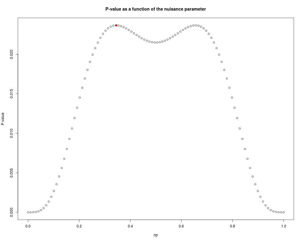
> data<-matrix(c(4,0,3,7),2,2,dimnames=list(c("Box 1","Box 2"),c("Defective","Not Defective")))
> exact.test(data,method="CSM",alternative="two.sided")
$model
[1] "Binomial"

$method
[1] "CSM"

$alternative
[1] "two.sided"

$p.value
[1] 0.02365848

$test.statistic
[1] NA

$np
[1] 0.345219

$np.range
[1] 0.00001 0.99999

> 
> data<-matrix(c(6,8,4,3),2,2,byrow=TRUE)
> exact.test(data,model="Multinomial",alternative="less",method="Z-pooled")
$model
[1] "Multinomial"

$method
[1] "Z-pooled"

$alternative
[1] "less"

$p.value
[1] 0.3388144

$test.statistic
[1] -0.6179144

$np1
[1] 0.6666633

$np2
[1] 0.895615

$np1.range
[1] 0.00001 0.99999

$np2.range
[1] 0.00001 0.99999

> 
> 
> 
> 
> 
> 
> dev.off()
null device 
          1 
>