Plot set of pixels on grid

Description

plot plots a grid of pixels based on an object from pgrid or confreg.

Usage

## S3 method for class 'pgrid'
plot(x, set, col = "gray", add = FALSE,
  type = "confidence", ...)

Arguments

Details

If a vector of pixel indices is supplied to set, then those pixels will be colored col by this function and the type argument has no effect. On the other hand, if the set argument is of class confreg, then the function digs in to display either the confidence or complement set in the confreg object. In that case, type is used to decide which set to display.

Value

This function does not return anything; it only creates a new plot or modifies an existing plot.

Author(s)

Joshua French

Examples

library(SpatialTools)

# Example for exceedance regions

set.seed(10)
# Load data
data(sdata)
# Create prediction grid
pgrid <- create.pgrid(0, 1, 0, 1, nx = 26, ny = 26)
pcoords <- pgrid$pgrid
# Create design matrices
coords = cbind(sdata$x1, sdata$x2)
X <- cbind(1, coords)
Xp <- cbind(1, pcoords)

# Generate covariance matrices V, Vp, Vop using appropriate parameters for
# observed data and responses to be predicted
spcov <- cov.sp(coords = coords, sp.type = "exponential",
 sp.par = c(1, 1.5), error.var = 1/3, finescale.var = 0, pcoords = pcoords)

# Predict responses at pgrid locations
krige.obj <- krige.uk(y = as.vector(sdata$y), V = spcov$V, Vp = spcov$Vp,
 Vop = spcov$Vop, X = X, Xp = Xp, nsim = 100,
 Ve.diag = rep(1/3, length(sdata$y)) , method = "chol")

# Simulate distribution of test statistic for different alternatives
statistic.sim.obj.less <- statistic.sim(krige.obj = krige.obj, level = 5,
 alternative = "less")
statistic.sim.obj.greater <- statistic.sim(krige.obj = krige.obj,
 level = 5, alternative = "greater")
# Construct null and rejection sets for two scenarios
n90 <- exceedance.ci(statistic.sim.obj.less, conf.level = .90,
 type = "null")
r90 <- exceedance.ci(statistic.sim.obj.greater,conf.level = .90,
 type = "rejection")
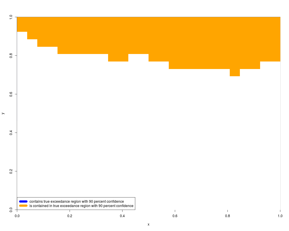
# Plot results
plot(pgrid, n90, col="blue", add = FALSE, xlab = "x", ylab = "y")
plot(pgrid, r90, col="orange", add = TRUE)
legend("bottomleft",
 legend = c("contains true exceedance region with 90 percent confidence",
 "is contained in true exceedance region with 90 percent confidence"),
 col = c("blue", "orange"), lwd = 10)

Results

R version 3.3.1 (2016-06-21) -- "Bug in Your Hair"
Copyright (C) 2016 The R Foundation for Statistical Computing
Platform: x86_64-pc-linux-gnu (64-bit)

R is free software and comes with ABSOLUTELY NO WARRANTY.
You are welcome to redistribute it under certain conditions.
Type 'license()' or 'licence()' for distribution details.

R is a collaborative project with many contributors.
Type 'contributors()' for more information and
'citation()' on how to cite R or R packages in publications.

Type 'demo()' for some demos, 'help()' for on-line help, or
'help.start()' for an HTML browser interface to help.
Type 'q()' to quit R.

> library(ExceedanceTools)
> png(filename="/home/ddbj/snapshot/RGM3/R_CC/result/ExceedanceTools/plot.pgrid.Rd_%03d_medium.png", width=480, height=480)
> ### Name: plot.pgrid
> ### Title: Plot set of pixels on grid
> ### Aliases: plot.pgrid
> 
> ### ** Examples
> 
> library(SpatialTools)
# This research was partially supported under NSF Grant ATM-0534173
> 
> # Example for exceedance regions
> 
> set.seed(10)
> # Load data
> data(sdata)
> # Create prediction grid
> pgrid <- create.pgrid(0, 1, 0, 1, nx = 26, ny = 26)
> pcoords <- pgrid$pgrid
> # Create design matrices
> coords = cbind(sdata$x1, sdata$x2)
> X <- cbind(1, coords)
> Xp <- cbind(1, pcoords)
> 
> # Generate covariance matrices V, Vp, Vop using appropriate parameters for
> # observed data and responses to be predicted
> spcov <- cov.sp(coords = coords, sp.type = "exponential",
+  sp.par = c(1, 1.5), error.var = 1/3, finescale.var = 0, pcoords = pcoords)
> 
> # Predict responses at pgrid locations
> krige.obj <- krige.uk(y = as.vector(sdata$y), V = spcov$V, Vp = spcov$Vp,
+  Vop = spcov$Vop, X = X, Xp = Xp, nsim = 100,
+  Ve.diag = rep(1/3, length(sdata$y)) , method = "chol")
> 
> # Simulate distribution of test statistic for different alternatives
> statistic.sim.obj.less <- statistic.sim(krige.obj = krige.obj, level = 5,
+  alternative = "less")
> statistic.sim.obj.greater <- statistic.sim(krige.obj = krige.obj,
+  level = 5, alternative = "greater")
> # Construct null and rejection sets for two scenarios
> n90 <- exceedance.ci(statistic.sim.obj.less, conf.level = .90,
+  type = "null")
> r90 <- exceedance.ci(statistic.sim.obj.greater,conf.level = .90,
+  type = "rejection")
> # Plot results
> plot(pgrid, n90, col="blue", add = FALSE, xlab = "x", ylab = "y")
> plot(pgrid, r90, col="orange", add = TRUE)
> legend("bottomleft",
+  legend = c("contains true exceedance region with 90 percent confidence",
+  "is contained in true exceedance region with 90 percent confidence"),
+  col = c("blue", "orange"), lwd = 10)
> 
> 
> 
> 
> 
> dev.off()
null device 
          1 
>