R Graphical Manual

Browse All

Last data update: 2014.03.03

R: The four-parameter beta distribution.

Beta_ab

R Documentation

The four-parameter beta distribution.

Description

Density, distribution, quantile, random number generation, and parameter estimation functions for the 4-parameter beta distribution. Parameter estimation can be based on a weighted or unweighted i.i.d sample and can be performed numerically.

Usage

dBeta_ab(x, shape1 = 2, shape2 = 3, a = 0, b = 1,
  params = list(shape1, shape2, a, b), ...)

pBeta_ab(q, shape1 = 2, shape2 = 3, a = 0, b = 1, params = list(shape1
  = 2, shape2 = 5, a = 0, b = 1), ...)

qBeta_ab(p, shape1 = 2, shape2 = 3, a = 0, b = 1, params = list(shape1
  = 2, shape2 = 5, a = 0, b = 1), ...)

rBeta_ab(n, shape1 = 2, shape2 = 3, a = 0, b = 1,
  params = list(shape1, shape2, a, b), ...)

eBeta_ab(X, w, method = "numerical.MLE", ...)

lBeta_ab(X, w, shape1 = 2, shape2 = 3, a = 0, b = 1,
  params = list(shape1, shape2, a, b), logL = TRUE, ...)

sBeta_ab(X, w, shape1 = 2, shape2 = 3, a = 0, b = 1,
  params = list(shape1, shape2, a, b), ...)

Arguments

`x,q`	A vector of quantiles.
`shape1,shape2`	Shape parameters.
`a,b`	Boundary parameters.
`params`	A list that includes all named parameters.
`...`	Additional parameters.
`p`	A vector of probabilities.
`n`	Number of observations.
`X`	Sample observations.
`w`	An optional vector of sample weights.
`method`	Parameter estimation method.
`logL`	logical; if TRUE, lBeta_ab gives the log-likelihood, otherwise the likelihood is given.

Details

The dBeta_ab(), pBeta_ab(), qBeta_ab(),and rBeta_ab() functions serve as wrappers of the standard dbeta, pbeta, qbeta and rbeta functions in the stats package.They allow for the parameters to be declared not only as individual numerical values, but also as a list so parameter estimation can be carried out.

The four-parameter beta distribution with parameters shape1=p, shape2=q, a = a and b=b has probability density function

f(x) = frac{1}{B(p,q)} frac{(x-a)^{(p-1)})(b-x)^{(q-1)}}{((b-a)^{(p+q-1)}))}

with p >0, q > 0, a ≤q x ≤q b and where B is the beta function, Johnson et.al (p.210).

The log-likelihood function of the four-parameter beta distribution is

l(p,q,a,b| x) = -ln B(p,q) + ((p-1) ln (x-a) + (q-1) ln (b-x)) - (p + q -1) ln (b-a).

Johnson et.al (p.226) provides the Fisher's information matrix of the four-parameter beta distribution in the regular case where p,q > 2.

Value

dBeta_ab gives the density, pBeta_ab the distribution function, qBeta_ab the quantile function, rBeta_ab generates random deviates, and eBeta_ab estimates the parameters. lBeta_ab provides the log-likelihood function, sBeta_ab the observed score function and iBeta_ab the observed information matrix.

Author(s)

Haizhen Wu and A. Jonathan R. Godfrey
Updates and bug fixes by Sarah Pirikahu.

References

Johnson, N. L., Kotz, S. and Balakrishnan, N. (1995) Continuous Univariate Distributions, volume 2, chapter 25, Wiley, New York.

Bury, K. (1999) Statistical Distributions in Engineering, Chapter 14, pp.261-262, Cambridge University Press.

Examples

# Parameter estimation for a distribution with known shape parameters
X <- rBeta_ab(n=500, shape1=2, shape2=5, a=1, b=2)
est.par <- eBeta_ab(X); est.par
plot(est.par)

# Fitted density curve and histogram
den.x <- seq(min(X),max(X),length=100)
den.y <- dBeta_ab(den.x,params = est.par)
hist(X, breaks=10, probability=TRUE, ylim = c(0,1.1*max(den.y)))
lines(den.x, den.y, col="blue")   # Original data
lines(density(X), lty=2)          # Fitted density curve

# Extracting boundary and shape parameters
est.par[attributes(est.par)$par.type=="boundary"]
est.par[attributes(est.par)$par.type=="shape"]

# Parameter Estimation for a distribution with unknown shape parameters
# Example from: Bury(1999) pp.261-262, parameter estimates as given by Bury are
# shape1 = 4.088, shape2 = 10.417, a = 1.279 and b = 2.407.
# The log-likelihood for this data and Bury's parameter estimates is 8.598672.
data <- c(1.73, 1.5, 1.56, 1.89, 1.54, 1.68, 1.39, 1.64, 1.49, 1.43, 1.68, 1.61, 1.62)
est.par <- eBeta_ab(X=data, method="numerical.MLE");est.par
plot(est.par)

# Estimates calculated by eBeta_ab differ from those given by Bury(1999).
# However, eBeta_ab's parameter estimates appear to be an improvement, due to a larger
# log-likelihood of 9.295922 (as given by lBeta_ab below).

# log-likelihood and score functions
lBeta_ab(data,param = est.par)
sBeta_ab(data,param = est.par)

Results


R version 3.3.1 (2016-06-21) -- "Bug in Your Hair"
Copyright (C) 2016 The R Foundation for Statistical Computing
Platform: x86_64-pc-linux-gnu (64-bit)

R is free software and comes with ABSOLUTELY NO WARRANTY.
You are welcome to redistribute it under certain conditions.
Type 'license()' or 'licence()' for distribution details.

R is a collaborative project with many contributors.
Type 'contributors()' for more information and
'citation()' on how to cite R or R packages in publications.

Type 'demo()' for some demos, 'help()' for on-line help, or
'help.start()' for an HTML browser interface to help.
Type 'q()' to quit R.

> library(ExtDist)

Attaching package: 'ExtDist'

The following object is masked from 'package:stats':

    BIC

> png(filename="/home/ddbj/snapshot/RGM3/R_CC/result/ExtDist/Beta_ab.Rd_%03d_medium.png", width=480, height=480)
> ### Name: Beta_ab
> ### Title: The four-parameter beta distribution.
> ### Aliases: Beta_ab dBeta_ab eBeta_ab lBeta_ab pBeta_ab qBeta_ab rBeta_ab
> ###   sBeta_ab
> 
> ### ** Examples
> 
> # Parameter estimation for a distribution with known shape parameters
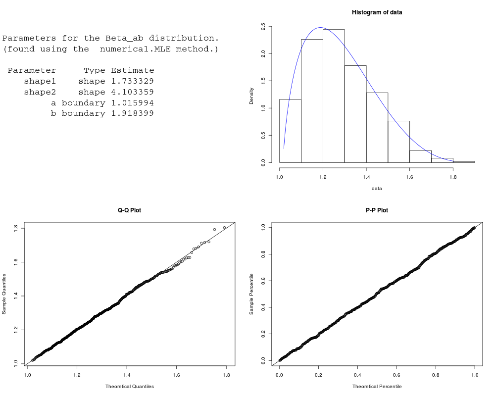
> X <- rBeta_ab(n=500, shape1=2, shape2=5, a=1, b=2)
> est.par <- eBeta_ab(X); est.par

Parameters for the Beta_ab distribution. 
(found using the  numerical.MLE method.)

 Parameter     Type Estimate
    shape1    shape 1.959611
    shape2    shape 4.106372
         a boundary 1.000596
         b boundary 1.866421


> plot(est.par)
> 
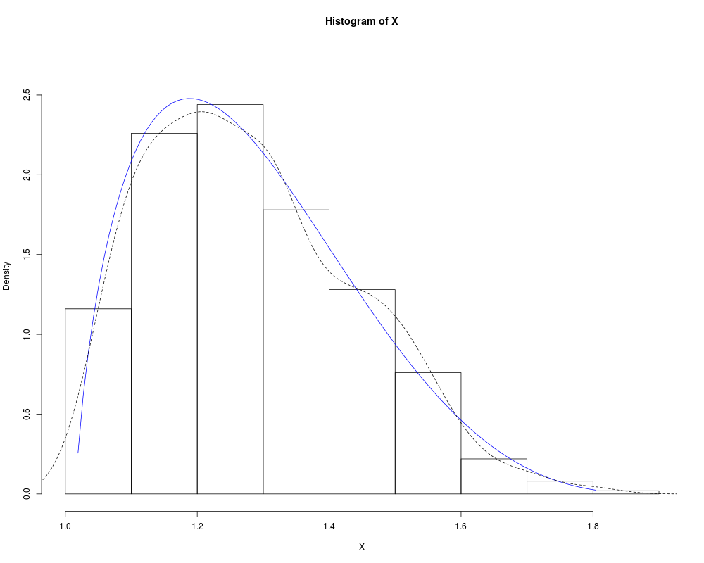
> # Fitted density curve and histogram
> den.x <- seq(min(X),max(X),length=100)
> den.y <- dBeta_ab(den.x,params = est.par)
> hist(X, breaks=10, probability=TRUE, ylim = c(0,1.1*max(den.y)))
> lines(den.x, den.y, col="blue")   # Original data
> lines(density(X), lty=2)          # Fitted density curve
> 
> # Extracting boundary and shape parameters
> est.par[attributes(est.par)$par.type=="boundary"]
$a
[1] 1.000596

$b
[1] 1.866421

> est.par[attributes(est.par)$par.type=="shape"]
$shape1
[1] 1.959611

$shape2
[1] 4.106372

> 
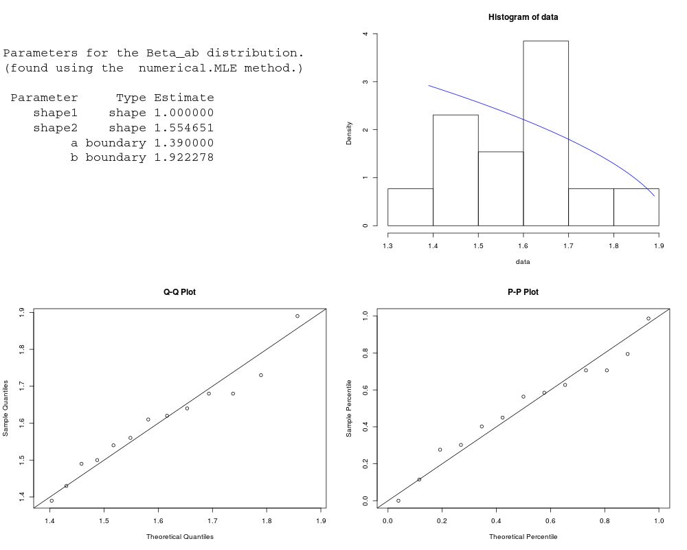
> # Parameter Estimation for a distribution with unknown shape parameters
> # Example from: Bury(1999) pp.261-262, parameter estimates as given by Bury are
> # shape1 = 4.088, shape2 = 10.417, a = 1.279 and b = 2.407.
> # The log-likelihood for this data and Bury's parameter estimates is 8.598672.
> data <- c(1.73, 1.5, 1.56, 1.89, 1.54, 1.68, 1.39, 1.64, 1.49, 1.43, 1.68, 1.61, 1.62)
> est.par <- eBeta_ab(X=data, method="numerical.MLE");est.par
Error in eigen(nhatend) : infinite or missing values in 'x'

Parameters for the Beta_ab distribution. 
(found using the  numerical.MLE method.)

 Parameter     Type Estimate
    shape1    shape 1.000000
    shape2    shape 1.554651
         a boundary 1.390000
         b boundary 1.922278


> plot(est.par)
> 
> # Estimates calculated by eBeta_ab differ from those given by Bury(1999).
> # However, eBeta_ab's parameter estimates appear to be an improvement, due to a larger
> # log-likelihood of 9.295922 (as given by lBeta_ab below).
> 
> # log-likelihood and score functions
> lBeta_ab(data,param = est.par)
[1] 9.295922
> sBeta_ab(data,param = est.par)
       shape1        shape2             a             b 
-1.867808e+01 -2.761777e-05  2.034795e+01  3.820333e-04 
> 
> 
> 
> 
> 
> dev.off()
null device 
          1 
>