The Exponential Distribution.

Description

Density, distribution, quantile, random number generation and parameter estimation functions for the exponential distribution. Parameter estimation can be based on a weighted or unweighted i.i.d sample and is carried out analytically.

Usage

dExp(x, scale = 1, params = list(scale = 1), ...)

pExp(q, scale = 1, params = list(scale = 1), ...)

qExp(p, scale = 1, params = list(scale = 1), ...)

rExp(n, scale = 1, params = list(scale = 1), ...)

eExp(x, w, method = "analytical.MLE", ...)

lExp(x, w, scale = 1, params = list(scale = 1), logL = TRUE, ...)

sExp(x, w, scale = 1, params = list(scale = 1), ...)

iExp(x, w, scale = 1, params = list(scale = 1), ...)

Arguments

Details

If scale is omitted, it assumes the default value 1 giving the standard exponential distribution.

The exponential distribution is a special case of the gamma distribution where the shape parameter α = 1. The dExp(), pExp(), qExp(),and rExp() functions serve as wrappers of the standard dexp, pexp, qexp and rexp functions in the stats package. They allow for the parameters to be declared not only as individual numerical values, but also as a list so parameter estimation can be carried out.

The probability density function for the exponential distribution with scale=β is

f(x) = (1/β) * exp(-x/β)

for β > 0 , Johnson et.al (Chapter 19, p.494). Parameter estimation for the exponential distribution is carried out analytically using maximum likelihood estimation (p.506 Johnson et.al).

The likelihood function of the exponential distribution is given by

l(λ|x) = n log λ - λ ∑ xi.

It follows that the score function is given by

dl(λ|x)/dλ = n/λ - ∑ xi

and Fisher's information given by

E[-d^2l(λ|x)/dλ^2] = n/λ^2.

Value

dExp gives the density, pExp the distribution function, qExp the quantile function, rExp generates random deviates, and eExp estimates the distribution parameters. lExp provides the log-likelihood function.

Author(s)

Jonathan R. Godfrey and Sarah Pirikahu.

References

Johnson, N. L., Kotz, S. and Balakrishnan, N. (1995) Continuous Univariate Distributions, volume 1, chapter 19, Wiley, New York.

Kapadia. A.S., Chan, W. and Moye, L. (2005) Mathematical Statistics with Applications, Chapter 8, Chapman& Hall/CRC.

Examples

# Parameter estimation for a distribution with known shape parameters
x <- rExp(n=500, scale=2)
est.par <- eExp(x); est.par
plot(est.par)

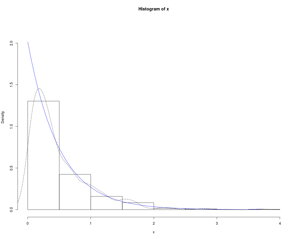
#  Fitted density curve and histogram
den.x <- seq(min(x),max(x),length=100)
den.y <- dExp(den.x,scale=est.par$scale)
hist(x, breaks=10, probability=TRUE, ylim = c(0,1.1*max(den.y)))
lines(den.x, den.y, col="blue")
lines(density(x), lty=2)

# Extracting the scale parameter
est.par[attributes(est.par)$par.type=="scale"]

# Parameter estimation for a distribution with unknown shape parameters
# Example from Kapadia et.al(2005), pp.380-381.
# Parameter estimate as given by Kapadia et.al is scale=0.00277
cardio <- c(525, 719, 2880, 150, 30, 251, 45, 858, 15,
           47, 90, 56, 68, 6, 139, 180, 60, 60, 294, 747)
est.par <- eExp(cardio, method="analytical.MLE"); est.par
plot(est.par)

# log-likelihood, score function and Fisher's information
lExp(cardio,param = est.par)
sExp(cardio,param = est.par)
iExp(cardio,param = est.par)

Results

R version 3.3.1 (2016-06-21) -- "Bug in Your Hair"
Copyright (C) 2016 The R Foundation for Statistical Computing
Platform: x86_64-pc-linux-gnu (64-bit)

R is free software and comes with ABSOLUTELY NO WARRANTY.
You are welcome to redistribute it under certain conditions.
Type 'license()' or 'licence()' for distribution details.

R is a collaborative project with many contributors.
Type 'contributors()' for more information and
'citation()' on how to cite R or R packages in publications.

Type 'demo()' for some demos, 'help()' for on-line help, or
'help.start()' for an HTML browser interface to help.
Type 'q()' to quit R.

> library(ExtDist)

Attaching package: 'ExtDist'

The following object is masked from 'package:stats':

    BIC

> png(filename="/home/ddbj/snapshot/RGM3/R_CC/result/ExtDist/Exponential.Rd_%03d_medium.png", width=480, height=480)
> ### Name: Exponential
> ### Title: The Exponential Distribution.
> ### Aliases: Exponential dExp eExp iExp lExp pExp qExp rExp sExp
> 
> ### ** Examples
> 
> # Parameter estimation for a distribution with known shape parameters
> x <- rExp(n=500, scale=2)
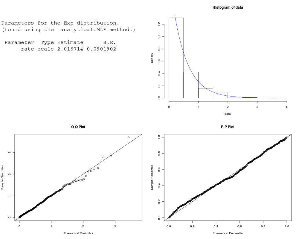
> est.par <- eExp(x); est.par

Parameters for the Exp distribution. 
(found using the  analytical.MLE method.)

 Parameter  Type Estimate       S.E.
      rate scale 2.028994 0.09073936


> plot(est.par)
> 
> #  Fitted density curve and histogram
> den.x <- seq(min(x),max(x),length=100)
> den.y <- dExp(den.x,scale=est.par$scale)
> hist(x, breaks=10, probability=TRUE, ylim = c(0,1.1*max(den.y)))
> lines(den.x, den.y, col="blue")
> lines(density(x), lty=2)
> 
> # Extracting the scale parameter
> est.par[attributes(est.par)$par.type=="scale"]
$scale
[1] 2.028994

> 
> # Parameter estimation for a distribution with unknown shape parameters
> # Example from Kapadia et.al(2005), pp.380-381.
> # Parameter estimate as given by Kapadia et.al is scale=0.00277
> cardio <- c(525, 719, 2880, 150, 30, 251, 45, 858, 15,
+            47, 90, 56, 68, 6, 139, 180, 60, 60, 294, 747)
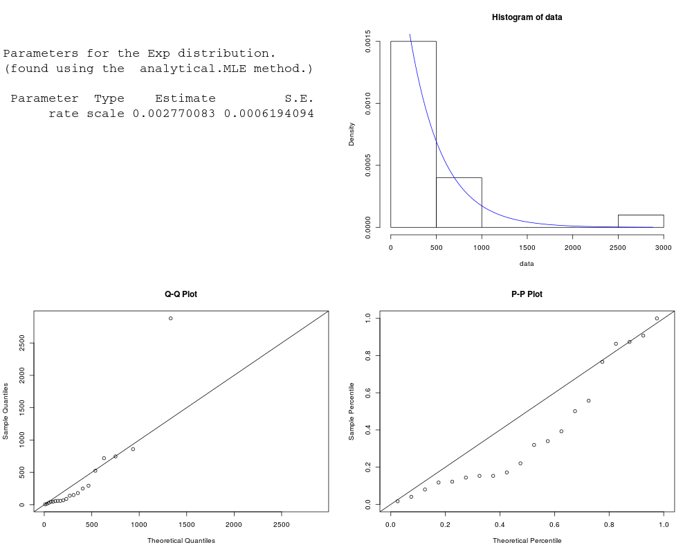
> est.par <- eExp(cardio, method="analytical.MLE"); est.par

Parameters for the Exp distribution. 
(found using the  analytical.MLE method.)

 Parameter  Type    Estimate         S.E.
      rate scale 0.002770083 0.0006194094


> plot(est.par)
> 
> # log-likelihood, score function and Fisher's information
> lExp(cardio,param = est.par)
[1] -137.7776
> sExp(cardio,param = est.par)
[1] 0
> iExp(cardio,param = est.par)
[1] 2606420
> 
> 
> 
> 
> 
> dev.off()
null device 
          1 
>