The Gamma Distribution.

Description

Density, distribution, quantile, random number generation, and parameter estimation functions for the gamma distribution with parameters shape and scale. Parameter estimation can be based on a weighted or unweighted i.i.d sample and can be carried out numerically.

Usage

dGamma(x, shape = 2, scale = 2, params = list(shape = 2, scale = 2), ...)

pGamma(q, shape = 2, scale = 2, params = list(shape = 2, scale = 2), ...)

qGamma(p, shape = 2, scale = 2, params = list(shape = 2, scale = 2), ...)

rGamma(n, shape = 2, scale = 2, params = list(shape = 2, scale = 2), ...)

eGamma(X, w, method = c("moments", "numerical.MLE"), ...)

lGamma(X, w, shape = 2, scale = 2, params = list(shape = 2, scale = 2),
  logL = TRUE, ...)

Arguments

Details

The dGamma(), pGamma(), qGamma(),and rGamma() functions serve as wrappers of the standard dgamma, pgamma, qgamma, and rgamma functions in the stats package. They allow for the parameters to be declared not only as individual numerical values, but also as a list so parameter estimation can be carried out.

The gamma distribution with parameter shape=α and scale=β has probability density function,

f(x)= (1/β^α Γ(α))x^{α-1}e^{-x/β}

where α > 0 and β > 0. Parameter estimation can be performed using the method of moments as given by Johnson et.al (pp.356-357).

The log-likelihood function of the gamma distribution is given by,

l(α, β |x) = (α -1) ∑_i ln(x_i) - ∑_i(x_i/β) -nα ln(β) + n ln Γ(α)

where Γ is the gamma function. The score function is provided by Rice (2007), p.270.

Value

dGamma gives the density, pGamma the distribution function, qGamma the quantile function, rGamma generates random deviates, and eGamma estimates the distribution parameters.lgamma provides the log-likelihood function.

Author(s)

Haizhen Wu and A. Jonathan R. Godfrey.
Updates and bug fixes by Sarah Pirikahu.

References

Johnson, N. L., Kotz, S. and Balakrishnan, N. (1995) Continuous Univariate Distributions, volume 1, chapter 17, Wiley, New York.

Bury, K. (1999) Statistical Distributions in Engineering, Chapter 13, pp.225-226, Cambridge University Press.

Rice, J.A. (2007) Mathematical Statistics and Data Analysis, 3rd Ed, Brookes/Cole.

See Also

ExtDist for other standard distributions.

Examples

# Parameter estimation for a distribution with known shape parameters
X <- rGamma(n=500, shape=1.5, scale=0.5)
est.par <- eGamma(X); est.par
plot(est.par)

#  Fitted density curve and histogram
den.x <- seq(min(X),max(X),length=100)
den.y <- dGamma(den.x,shape=est.par$shape,scale=est.par$scale)
hist(X, breaks=10, probability=TRUE, ylim = c(0,1.1*max(den.y)))
lines(den.x, den.y, col="blue")
lines(density(X), lty=2)

# Extracting shape or scale parameters
est.par[attributes(est.par)$par.type=="shape"]
est.par[attributes(est.par)$par.type=="scale"]

# Parameter estimation for a distribution with unknown shape parameters
# Example from:  Bury(1999) pp.225-226, parameter estimates as given by Bury are
# shape = 6.40 and scale=2.54. The log-likelihood for this data given
# Bury's parameter estimates is -656.7921.
data <- c(16, 11.6, 19.9, 18.6, 18, 13.1, 29.1, 10.3, 12.2, 15.6, 12.7, 13.1,
         19.2, 19.5, 23, 6.7, 7.1, 14.3, 20.6, 25.6, 8.2, 34.4, 16.1, 10.2, 12.3)
est.par <- eGamma(data, method="numerical.MLE"); est.par
plot(est.par)

# Estimates calculated by eGamma differ from those given by Bury(1999).
# However, eGamma's parameter estimates appear to be an improvement, due to a larger
# log-likelihood of -80.68186 (as given by lGamma below).

# log-likelihood
lGamma(data,param = est.par)

# Evaluating the precision of the parameter estimates by the Hessian matrix
H <- attributes(est.par)$nll.hessian
var <- solve(H)
se <- sqrt(diag(var));se

Results

R version 3.3.1 (2016-06-21) -- "Bug in Your Hair"
Copyright (C) 2016 The R Foundation for Statistical Computing
Platform: x86_64-pc-linux-gnu (64-bit)

R is free software and comes with ABSOLUTELY NO WARRANTY.
You are welcome to redistribute it under certain conditions.
Type 'license()' or 'licence()' for distribution details.

R is a collaborative project with many contributors.
Type 'contributors()' for more information and
'citation()' on how to cite R or R packages in publications.

Type 'demo()' for some demos, 'help()' for on-line help, or
'help.start()' for an HTML browser interface to help.
Type 'q()' to quit R.

> library(ExtDist)

Attaching package: 'ExtDist'

The following object is masked from 'package:stats':

    BIC

> png(filename="/home/ddbj/snapshot/RGM3/R_CC/result/ExtDist/Gamma.Rd_%03d_medium.png", width=480, height=480)
> ### Name: Gamma
> ### Title: The Gamma Distribution.
> ### Aliases: Gamma dGamma eGamma lGamma pGamma qGamma rGamma
> 
> ### ** Examples
> 
> # Parameter estimation for a distribution with known shape parameters
> X <- rGamma(n=500, shape=1.5, scale=0.5)
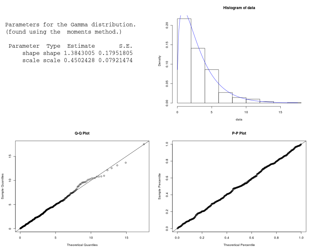
> est.par <- eGamma(X); est.par

Parameters for the Gamma distribution. 
(found using the  moments method.)

 Parameter  Type  Estimate      S.E.
     shape shape 1.5881838 0.1564567
     scale scale 0.5464532 0.0918294


> plot(est.par)
> 
> #  Fitted density curve and histogram
> den.x <- seq(min(X),max(X),length=100)
> den.y <- dGamma(den.x,shape=est.par$shape,scale=est.par$scale)
> hist(X, breaks=10, probability=TRUE, ylim = c(0,1.1*max(den.y)))
> lines(den.x, den.y, col="blue")
> lines(density(X), lty=2)
> 
> # Extracting shape or scale parameters
> est.par[attributes(est.par)$par.type=="shape"]
$shape
[1] 1.588184

> est.par[attributes(est.par)$par.type=="scale"]
$scale
[1] 0.5464532

> 
> # Parameter estimation for a distribution with unknown shape parameters
> # Example from:  Bury(1999) pp.225-226, parameter estimates as given by Bury are
> # shape = 6.40 and scale=2.54. The log-likelihood for this data given
> # Bury's parameter estimates is -656.7921.
> data <- c(16, 11.6, 19.9, 18.6, 18, 13.1, 29.1, 10.3, 12.2, 15.6, 12.7, 13.1,
+          19.2, 19.5, 23, 6.7, 7.1, 14.3, 20.6, 25.6, 8.2, 34.4, 16.1, 10.2, 12.3)
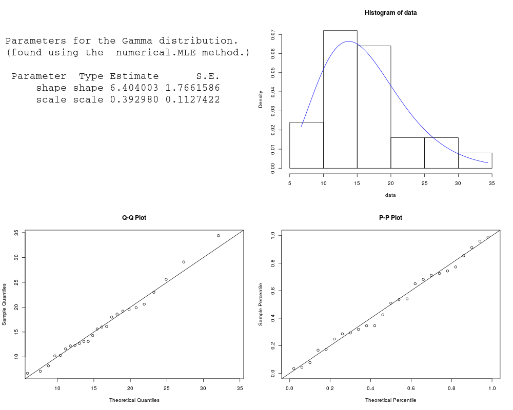
> est.par <- eGamma(data, method="numerical.MLE"); est.par

Parameters for the Gamma distribution. 
(found using the  numerical.MLE method.)

 Parameter  Type Estimate      S.E.
     shape shape 6.404003 1.7661586
     scale scale 0.392980 0.1127422


> plot(est.par)
> 
> # Estimates calculated by eGamma differ from those given by Bury(1999).
> # However, eGamma's parameter estimates appear to be an improvement, due to a larger
> # log-likelihood of -80.68186 (as given by lGamma below).
> 
> # log-likelihood
> lGamma(data,param = est.par)
[1] -80.68186
> 
> # Evaluating the precision of the parameter estimates by the Hessian matrix
> H <- attributes(est.par)$nll.hessian
> var <- solve(H)
> se <- sqrt(diag(var));se
    shape     scale 
1.7661586 0.1127422 
> 
> 
> 
> 
> 
> dev.off()
null device 
          1 
>