Supported by Dr. Osamu Ogasawara and  . . |
|
Last data update: 2014.03.03 |
The Johnson SB distribution.DescriptionDensity, distribution, quantile, random number generation, and parameter estimation functions for the Johnson SB (bounded support) distribution. Parameter estimation can be based on a weighted or unweighted i.i.d. sample and can be performed numerically. UsagedJohnsonSB(x, gamma = -0.5, delta = 2, xi = -0.5, lambda = 2, params = list(gamma = -0.5, delta = 2, xi = -0.5, lambda = 2), ...) dJohnsonSB_ab(x, gamma = -0.5, delta = 2, a = -0.5, b = 1.5, params = list(gamma = -0.5, delta = 2, a = -0.5, b = 1.5), ...) pJohnsonSB(q, gamma = -0.5, delta = 2, xi = -0.5, lambda = 2, params = list(gamma = -0.5, delta = 2, xi = -0.5, lambda = 2), ...) qJohnsonSB(p, gamma = -0.5, delta = 2, xi = -0.5, lambda = 2, params = list(gamma = -0.5, delta = 2, xi = -0.5, lambda = 2), ...) rJohnsonSB(n, gamma = -0.5, delta = 2, xi = -0.5, lambda = 2, params = list(gamma = -0.5, delta = 2, xi = -0.5, lambda = 2), ...) eJohnsonSB(X, w, method = "numerical.MLE", ...) lJohnsonSB(X, w, gamma = -0.5, delta = 2, xi = -0.5, lambda = 2, params = list(gamma = -0.5, delta = 2, xi = -0.5, lambda = 2), logL = TRUE, ...) Arguments
DetailsThe Johnson system of distributions consists of families of distributions that, through specified transformations, can be reduced to the standard normal random variable. It provides a very flexible system for describing statistical distributions and is defined by z = γ + δ f(Y) with Y = (X-xi)/lambda. The Johnson SB distribution arises when f(Y) = ln[Y/(1-Y)], where 0 < Y < 1.
This is the bounded Johnson family since the range of Y is (0,1), Karian & Dudewicz (2011). p_X(x) = frac{δ lambda}{√{2π}(x-xi)(1- x + xi)}exp[-0.5(γ + δ ln((x-xi)/(1-x+xi)))^2]. ValuedJohnsonSB gives the density, pJohnsonSB the distribution function, qJohnsonSB gives quantile function, rJohnsonSB generates random deviates, and eJohnsonSB estimate the parameters. lJohnsonSB provides the log-likelihood function. The dJohnsonSB_ab provides an alternative parameterisation of the JohnsonSB distribution. Author(s)Haizhen Wu and A. Jonathan R. Godfrey. ReferencesJohnson, N. L., Kotz, S. and Balakrishnan, N. (1994) Continuous Univariate Distributions,
volume 1, chapter 12, Wiley, New York. See AlsoExtDist for other standard distributions. Examples
# Parameter estimation for a distribution with known shape parameters
X <- rJohnsonSB(n=500, gamma=-0.5, delta=2, xi=-0.5, lambda=2)
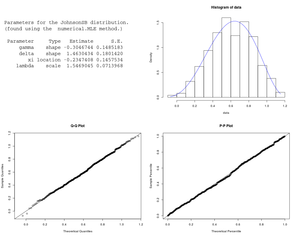
est.par <- eJohnsonSB(X); est.par
plot(est.par)
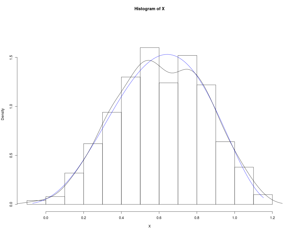
# Fitted density curve and histogram
den.x <- seq(min(X),max(X),length=100)
den.y <- dJohnsonSB(den.x,params = est.par)
hist(X, breaks=10, probability=TRUE, ylim = c(0,1.2*max(den.y)))
lines(den.x, den.y, col="blue")
lines(density(X))
# Extracting location, scale and shape parameters
est.par[attributes(est.par)$par.type=="location"]
est.par[attributes(est.par)$par.type=="scale"]
est.par[attributes(est.par)$par.type=="shape"]
# Parameter Estimation for a distribution with unknown shape parameters
# Example from Karian, Z.A and Dudewicz, E.J. (2011) p.647.
# Original source of brain scan data Dudewich, E.J et.al (1989).
# Parameter estimates as given by Karian & Dudewicz using moments are:
# gamma =-0.2081, delta=0.9167, xi = 95.1280 and lambda = 21.4607 with log-likelihood = -67.03579
brain <- c(108.7, 107.0, 110.3, 110.0, 113.6, 99.2, 109.8, 104.5, 108.1, 107.2, 112.0, 115.5, 108.4,
107.4, 113.4, 101.2, 98.4, 100.9, 100.0, 107.1, 108.7, 102.5, 103.3)
est.par <- eJohnsonSB(brain); est.par
# Estimates calculated by eJohnsonSB differ from those given by Karian & Dudewicz (2011).
# However, eJohnsonSB's parameter estimates appear to be an improvement, due to a larger
# log-likelihood of -66.35496 (as given by lJohnsonSB below).
# log-likelihood function
lJohnsonSB(brain, param = est.par)
Results
R version 3.3.1 (2016-06-21) -- "Bug in Your Hair"
Copyright (C) 2016 The R Foundation for Statistical Computing
Platform: x86_64-pc-linux-gnu (64-bit)

R is free software and comes with ABSOLUTELY NO WARRANTY.
You are welcome to redistribute it under certain conditions.
Type 'license()' or 'licence()' for distribution details.

R is a collaborative project with many contributors.
Type 'contributors()' for more information and
'citation()' on how to cite R or R packages in publications.

Type 'demo()' for some demos, 'help()' for on-line help, or
'help.start()' for an HTML browser interface to help.
Type 'q()' to quit R.

> library(ExtDist)

Attaching package: 'ExtDist'

The following object is masked from 'package:stats':

    BIC

> png(filename="/home/ddbj/snapshot/RGM3/R_CC/result/ExtDist/JohnsonSB.Rd_%03d_medium.png", width=480, height=480)
> ### Name: JohnsonSB
> ### Title: The Johnson SB distribution.
> ### Aliases: JohnsonSB dJohnsonSB dJohnsonSB_ab eJohnsonSB lJohnsonSB
> ###   pJohnsonSB qJohnsonSB rJohnsonSB
>
> ### ** Examples
>
> # Parameter estimation for a distribution with known shape parameters
> X <- rJohnsonSB(n=500, gamma=-0.5, delta=2, xi=-0.5, lambda=2)
> est.par <- eJohnsonSB(X); est.par

Parameters for the JohnsonSB distribution.
(found using the  numerical.MLE method.)

 Parameter     Type   Estimate       S.E.
     gamma    shape -0.6514553 0.33341362
     delta    shape  1.7284205 0.31462435
        xi location -0.4340878 0.30098015
    lambda    scale  1.7967701 0.09355422


> plot(est.par)
>
> #  Fitted density curve and histogram
> den.x <- seq(min(X),max(X),length=100)
> den.y <- dJohnsonSB(den.x,params = est.par)
> hist(X, breaks=10, probability=TRUE, ylim = c(0,1.2*max(den.y)))
> lines(den.x, den.y, col="blue")
> lines(density(X))
>
> # Extracting location, scale and shape parameters
> est.par[attributes(est.par)$par.type=="location"]
$xi
[1] -0.4340878

> est.par[attributes(est.par)$par.type=="scale"]
$lambda
[1] 1.79677

> est.par[attributes(est.par)$par.type=="shape"]
$gamma
[1] -0.6514553

$delta
[1] 1.728421

>
> # Parameter Estimation for a distribution with unknown shape parameters
> # Example from Karian, Z.A and Dudewicz, E.J. (2011) p.647.
> # Original source of brain scan data Dudewich, E.J et.al (1989).
> # Parameter estimates as given by Karian & Dudewicz using moments are:
> # gamma =-0.2081, delta=0.9167, xi = 95.1280 and lambda = 21.4607 with log-likelihood = -67.03579
> brain <- c(108.7, 107.0, 110.3, 110.0, 113.6, 99.2, 109.8, 104.5, 108.1, 107.2, 112.0, 115.5, 108.4,
+            107.4, 113.4, 101.2, 98.4, 100.9, 100.0, 107.1, 108.7, 102.5, 103.3)
> est.par <- eJohnsonSB(brain); est.par

Parameters for the JohnsonSB distribution.
(found using the  numerical.MLE method.)

 Parameter     Type   Estimate
     gamma    shape  0.0491309
     delta    shape  0.6547437
        xi location 97.9208050
    lambda    scale 18.0843462


>
> # Estimates calculated by eJohnsonSB differ from those given by Karian & Dudewicz (2011).
> # However, eJohnsonSB's parameter estimates appear to be an improvement, due to a larger
> # log-likelihood of -66.35496 (as given by lJohnsonSB below).
>
> # log-likelihood function
> lJohnsonSB(brain, param = est.par)
[1] -66.35496
>
>
>
>
>
> dev.off()
null device
          1
>
|