Supported by Dr. Osamu Ogasawara and  . . |
|
Last data update: 2014.03.03 |
The Johnson SU distribution.DescriptionDensity, distribution, quantile, random number generation and parameter estimation functions for the Johnson SU (unbounded support) distribution. Parameter estimation can be based on a weighted or unweighted i.i.d sample and can be carried out numerically. UsagedJohnsonSU(x, gamma = -0.5, delta = 2, xi = -0.5, lambda = 2, params = list(gamma = -0.5, delta = 2, xi = -0.5, lambda = 2), ...) pJohnsonSU(q, gamma = -0.5, delta = 2, xi = -0.5, lambda = 2, params = list(gamma = -0.5, delta = 2, xi = -0.5, lambda = 2), ...) qJohnsonSU(p, gamma = -0.5, delta = 2, xi = -0.5, lambda = 2, params = list(gamma = -0.5, delta = 2, xi = -0.5, lambda = 2), ...) rJohnsonSU(n, gamma = -0.5, delta = 2, xi = -0.5, lambda = 2, params = list(gamma = -0.5, delta = 2, xi = -0.5, lambda = 2), ...) eJohnsonSU(X, w, method = "numerical.MLE", ...) lJohnsonSU(X, w, gamma = -0.5, delta = 2, xi = -0.5, lambda = 2, params = list(gamma = -0.5, delta = 2, xi = -0.5, lambda = 2), logL = TRUE, ...) Arguments
DetailsThe Johnson system of distributions consists of families of distributions that, through specified transformations, can be reduced to the standard normal random variable. It provides a very flexible system for describing statistical distributions and is defined by z = γ + δ f(Y) with Y = (X-xi)/lambda. The Johnson SB distribution arises when f(Y) = archsinh(Y), where -∞ < Y < ∞.
This is the unbounded Johnson family since the range of Y is (-∞,∞), Karian & Dudewicz (2011). p_X(x) = frac{δ}{√{2π((x-xi)^2 + lambda^2)}}exp[-0.5(γ + δ ln(frac{x-xi + √{(x-xi)^2 + lambda^2}}{lambda}))^2]. Parameter estimation can only be carried out numerically. ValuedJohnsonSU gives the density, pJohnsonSU the distribution function, qJohnsonSU gives the quantile function, rJohnsonSU generates random variables, and eJohnsonSU estimates the parameters. lJohnsonSU provides the log-likelihood function. Author(s)Haizhen Wu and A. Jonathan R. Godfrey. ReferencesJohnson, N. L., Kotz, S. and Balakrishnan, N. (1994) Continuous Univariate Distributions,
volume 1, chapter 12, Wiley, New York. See AlsoExtDist for other standard distributions. Examples
# Parameter estimation for a known distribution
X <- rJohnsonSU(n=500, gamma=-0.5, delta=2, xi=-0.5, lambda=2)
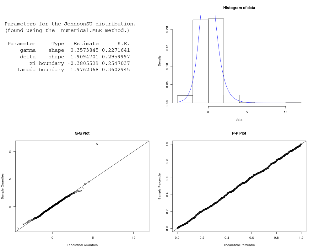
est.par <- eJohnsonSU(X); est.par
plot(est.par)
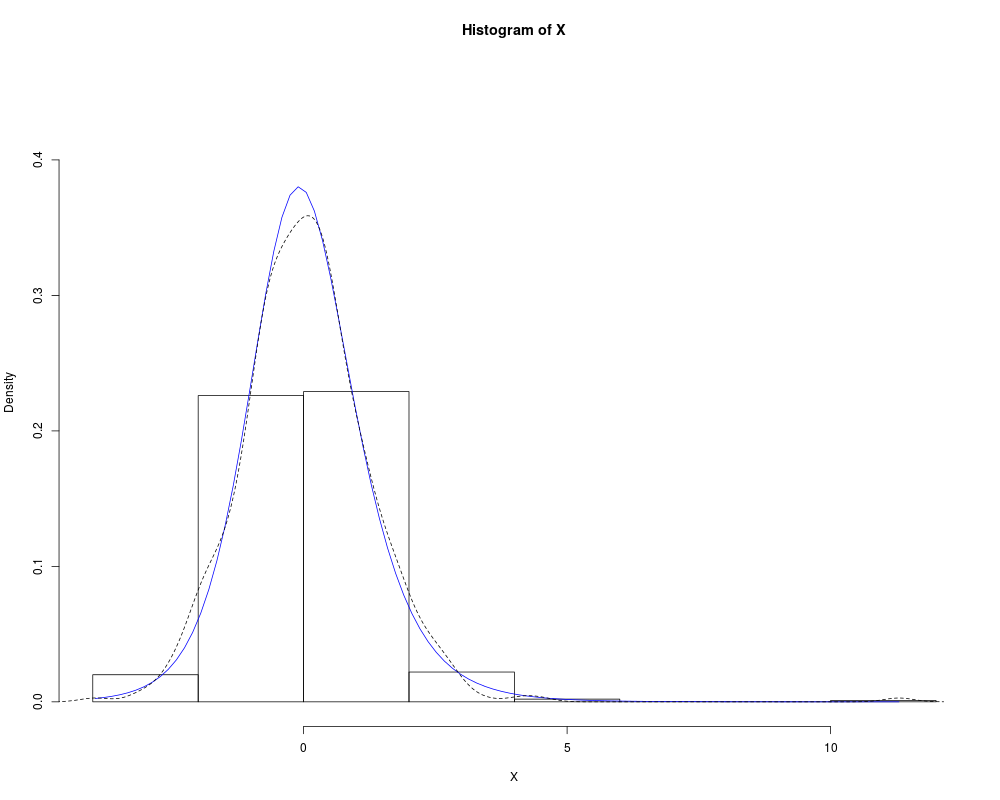
# Fitted density curve and histogram
den.x <- seq(min(X),max(X),length=100)
den.y <- dJohnsonSU(den.x,params = est.par)
hist(X, breaks=10, probability=TRUE, ylim = c(0,1.2*max(den.y)))
lines(den.x, den.y, col="blue")
lines(density(X), lty=2)
# Extracting shape and boundary parameters
est.par[attributes(est.par)$par.type=="shape"]
est.par[attributes(est.par)$par.type=="boundary"]
# Parameter Estimation for a distribution with unknown shape parameters
# Example from Karian, Z.A and Dudewicz, E.J. (2011) p.657.
# Parameter estimates as given by Karian & Dudewicz are:
# gamma =-0.2823, delta=1.0592, xi = -1.4475 and lambda = 4.2592 with log-likelihood = -277.1543
data <- c(1.99, -0.424, 5.61, -3.13, -2.24, -0.14, -3.32, -0.837, -1.98, -0.120,
7.81, -3.13, 1.20, 1.54, -0.594, 1.05, 0.192, -3.83, -0.522, 0.605,
0.427, 0.276, 0.784, -1.30, 0.542, -0.159, -1.66, -2.46, -1.81, -0.412,
-9.67, 6.61, -0.589, -3.42, 0.036, 0.851, -1.34, -1.22, -1.47, -0.592,
-0.311, 3.85, -4.92, -0.112, 4.22, 1.89, -0.382, 1.20, 3.21, -0.648,
-0.523, -0.882, 0.306, -0.882, -0.635, 13.2, 0.463, -2.60, 0.281, 1.00,
-0.336, -1.69, -0.484, -1.68, -0.131, -0.166, -0.266, 0.511, -0.198, 1.55,
-1.03, 2.15, 0.495, 6.37, -0.714, -1.35, -1.55, -4.79, 4.36, -1.53,
-1.51, -0.140, -1.10, -1.87, 0.095, 48.4, -0.998, -4.05, -37.9, -0.368,
5.25, 1.09, 0.274, 0.684, -0.105, 20.3, 0.311, 0.621, 3.28, 1.56)
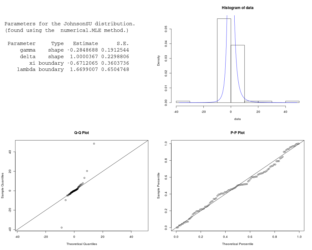
est.par <- eJohnsonSU(data); est.par
plot(est.par)
# Estimates calculated by eJohnsonSU differ from those given by Karian & Dudewicz (2011).
# However, eJohnsonSU's parameter estimates appear to be an improvement, due to a larger
# log-likelihood of -250.3208 (as given by lJohnsonSU below).
# log-likelihood function
lJohnsonSU(data, param = est.par)
# Evaluation of the precision using the Hessian matrix
H <- attributes(est.par)$nll.hessian
var <- solve(H)
se <- sqrt(diag(var)); se
Results
R version 3.3.1 (2016-06-21) -- "Bug in Your Hair"
Copyright (C) 2016 The R Foundation for Statistical Computing
Platform: x86_64-pc-linux-gnu (64-bit)

R is free software and comes with ABSOLUTELY NO WARRANTY.
You are welcome to redistribute it under certain conditions.
Type 'license()' or 'licence()' for distribution details.

R is a collaborative project with many contributors.
Type 'contributors()' for more information and
'citation()' on how to cite R or R packages in publications.

Type 'demo()' for some demos, 'help()' for on-line help, or
'help.start()' for an HTML browser interface to help.
Type 'q()' to quit R.

> library(ExtDist)

Attaching package: 'ExtDist'

The following object is masked from 'package:stats':

    BIC

> png(filename="/home/ddbj/snapshot/RGM3/R_CC/result/ExtDist/JohnsonSU.Rd_%03d_medium.png", width=480, height=480)
> ### Name: JohnsonSU
> ### Title: The Johnson SU distribution.
> ### Aliases: JohnsonSU dJohnsonSU eJohnsonSU lJohnsonSU pJohnsonSU
> ###   qJohnsonSU rJohnsonSU
>
> ### ** Examples
>
> # Parameter estimation for a known distribution
> X <- rJohnsonSU(n=500, gamma=-0.5, delta=2, xi=-0.5, lambda=2)
> est.par <- eJohnsonSU(X); est.par

Parameters for the JohnsonSU distribution.
(found using the  numerical.MLE method.)

 Parameter     Type   Estimate      S.E.
     gamma    shape -0.3939075 0.2184902
     delta    shape  1.8717867 0.3024863
        xi boundary -0.3630743 0.2206103
    lambda boundary  1.7450555 0.3347097


> plot(est.par)
>
> # Fitted density curve and histogram
> den.x <- seq(min(X),max(X),length=100)
> den.y <- dJohnsonSU(den.x,params = est.par)
> hist(X, breaks=10, probability=TRUE, ylim = c(0,1.2*max(den.y)))
> lines(den.x, den.y, col="blue")
> lines(density(X), lty=2)
>
> # Extracting shape and boundary parameters
> est.par[attributes(est.par)$par.type=="shape"]
$gamma
[1] -0.3939075

$delta
[1] 1.871787

> est.par[attributes(est.par)$par.type=="boundary"]
$xi
[1] -0.3630743

$lambda
[1] 1.745055

>
> # Parameter Estimation for a distribution with unknown shape parameters
> # Example from Karian, Z.A and Dudewicz, E.J. (2011) p.657.
> # Parameter estimates as given by Karian & Dudewicz are:
> # gamma =-0.2823, delta=1.0592, xi = -1.4475 and lambda = 4.2592  with log-likelihood = -277.1543
> data <- c(1.99, -0.424, 5.61, -3.13, -2.24, -0.14, -3.32, -0.837, -1.98, -0.120,
+          7.81, -3.13, 1.20, 1.54, -0.594, 1.05, 0.192, -3.83, -0.522, 0.605,
+          0.427, 0.276, 0.784, -1.30, 0.542, -0.159, -1.66, -2.46, -1.81, -0.412,
+          -9.67, 6.61, -0.589, -3.42, 0.036, 0.851, -1.34, -1.22, -1.47, -0.592,
+          -0.311, 3.85, -4.92, -0.112, 4.22, 1.89, -0.382, 1.20, 3.21, -0.648,
+          -0.523, -0.882, 0.306, -0.882, -0.635, 13.2, 0.463, -2.60, 0.281, 1.00,
+          -0.336, -1.69, -0.484, -1.68, -0.131, -0.166, -0.266, 0.511, -0.198, 1.55,
+          -1.03, 2.15, 0.495, 6.37, -0.714, -1.35, -1.55, -4.79, 4.36, -1.53,
+          -1.51, -0.140, -1.10, -1.87, 0.095, 48.4, -0.998, -4.05, -37.9, -0.368,
+          5.25, 1.09, 0.274, 0.684, -0.105, 20.3, 0.311, 0.621, 3.28, 1.56)
> est.par <- eJohnsonSU(data); est.par

Parameters for the JohnsonSU distribution.
(found using the  numerical.MLE method.)

 Parameter     Type   Estimate      S.E.
     gamma    shape -0.2848688 0.1912544
     delta    shape  1.0000367 0.2298806
        xi boundary -0.6712065 0.3603736
    lambda boundary  1.6699007 0.6504748


> plot(est.par)
>
> # Estimates calculated by eJohnsonSU differ from those given by Karian & Dudewicz (2011).
> # However, eJohnsonSU's parameter estimates appear to be an improvement, due to a larger
> # log-likelihood of -250.3208 (as given by lJohnsonSU below).
>
> # log-likelihood function
> lJohnsonSU(data, param = est.par)
[1] -250.3208
>
> # Evaluation of the precision using the Hessian matrix
> H <- attributes(est.par)$nll.hessian
> var <- solve(H)
> se <- sqrt(diag(var)); se
    gamma     delta        xi    lambda
0.1912544 0.2298806 0.3603736 0.6504748
>
>
>
>
>
> dev.off()
null device
          1
>
|