The Laplace Distribution.

Description

Density, distribution, quantile, random number generation and parameter estimation functions for the Laplace distribution with location parameter μ and scale parameter b. Parameter estimation can for the Laplace distribution can be carried out numerically or analytically but may only be based on an unweighted i.i.d. sample.

Usage

dLaplace(x, mu = 0, b = 1, params = list(mu, b), ...)

pLaplace(q, mu = 0, b = 1, params = list(mu, b), ...)

qLaplace(p, mu = 0, b = 1, params = list(mu, b), ...)

rLaplace(n, mu = 0, b = 1, params = list(mu, b), ...)

eLaplace(X, w, method = c("analytic.MLE", "numerical.MLE"), ...)

lLaplace(x, w = 1, mu = 0, b = 1, params = list(mu, b), logL = TRUE,
  ...)

Arguments

Details

The dLaplace(), pLaplace(), qLaplace(),and rLaplace() functions allow for the parameters to be declared not only as individual numerical values, but also as a list so parameter estimation can be carried out.

The Laplace distribution with parameters location = μ and scale=b has probability density function

f(x) = (1/2b) exp(-|x-μ|/b)

where -∞ < x < ∞ and b > 0. The cumulative distribution function for pLaplace is defined by Johnson et.al (p.166).

Parameter estimation can be carried out analytically via maximum likelihood estimation, see Johnson et.al (p.172). Where the population mean, μ, is estimated using the sample median and b by the mean of |x-b|.

Johnson et.al (p.172) also provides the log-likelihood function for the Laplace distribution

l(μ, b | x) = -n ln(2b) - b^{-1} ∑ |xi-μ|.

Value

dLaplace gives the density, pLaplace the distribution function, qLaplace the quantile function, rLaplace generates random deviates, and eLaplace estimates the distribution parameters. lLaplace provides the log-likelihood function, sLaplace the score function, and iLaplace the observed information matrix.

Note

The estimation of the population mean is done using the median of the sample. Unweighted samples are not yet catered for in the eLaplace() function.

Author(s)

A. Jonathan R. Godfrey and Haizhen Wu.
Updates and bug fixes by Sarah Pirikahu

References

Johnson, N. L., Kotz, S. and Balakrishnan, N. (1995) Continuous Univariate Distributions, volume 2, chapter 24, Wiley, New York.

Best, D.J., Rayner, J.C.W. and Thas O. (2008) Comparison of some tests of fit for the Laplace distribution, Computational Statistics and Data Analysis, Vol. 52, pp.5338-5343.

Gumbel, E.J., Mustafi, C.K., 1967. Some analytical properties of bivariate extremal distributions. J. Am. Stat. Assoc. 62, 569-588

See Also

ExtDist for other standard distributions.

Examples

# Parameter estimation for a distribution with known shape parameters
X <- rLaplace(n=500, mu=1, b=2)
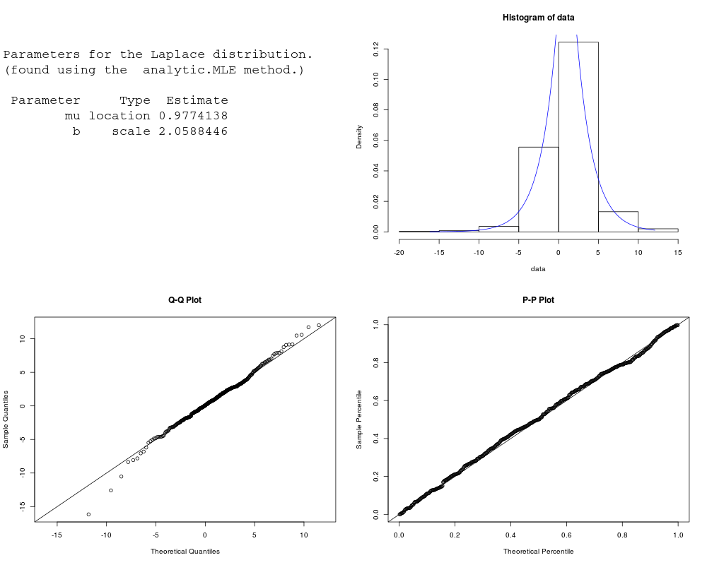
est.par <- eLaplace(X, method="analytic.MLE"); est.par
plot(est.par)

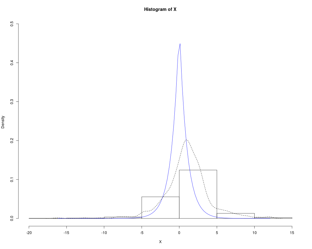
#  Fitted density curve and histogram
den.x <- seq(min(X),max(X),length=100)
den.y <- dLaplace(den.x, location = est.par$location, scale= est.par$scale)
hist(X, breaks=10, probability=TRUE, ylim = c(0,1.1*max(den.y)))
lines(den.x, den.y, col="blue")
lines(density(X), lty=2)

# Extracting location or scale parameters
est.par[attributes(est.par)$par.type=="location"]
est.par[attributes(est.par)$par.type=="scale"]

# Parameter estimation for a distribution with unknown shape parameters
# Example from Best et.al (2008). Original source of flood data from Gumbel & Mustafi.
# Parameter estimates as given by Best et.al mu=10.13 and  b=3.36
flood <- c(1.96, 1.96, 3.60, 3.80, 4.79, 5.66, 5.76, 5.78, 6.27, 6.30, 6.76, 7.65, 7.84, 7.99,
           8.51, 9.18, 10.13, 10.24, 10.25, 10.43, 11.45, 11.48, 11.75, 11.81, 12.34, 12.78, 13.06,
           13.29, 13.98, 14.18, 14.40, 16.22, 17.06)
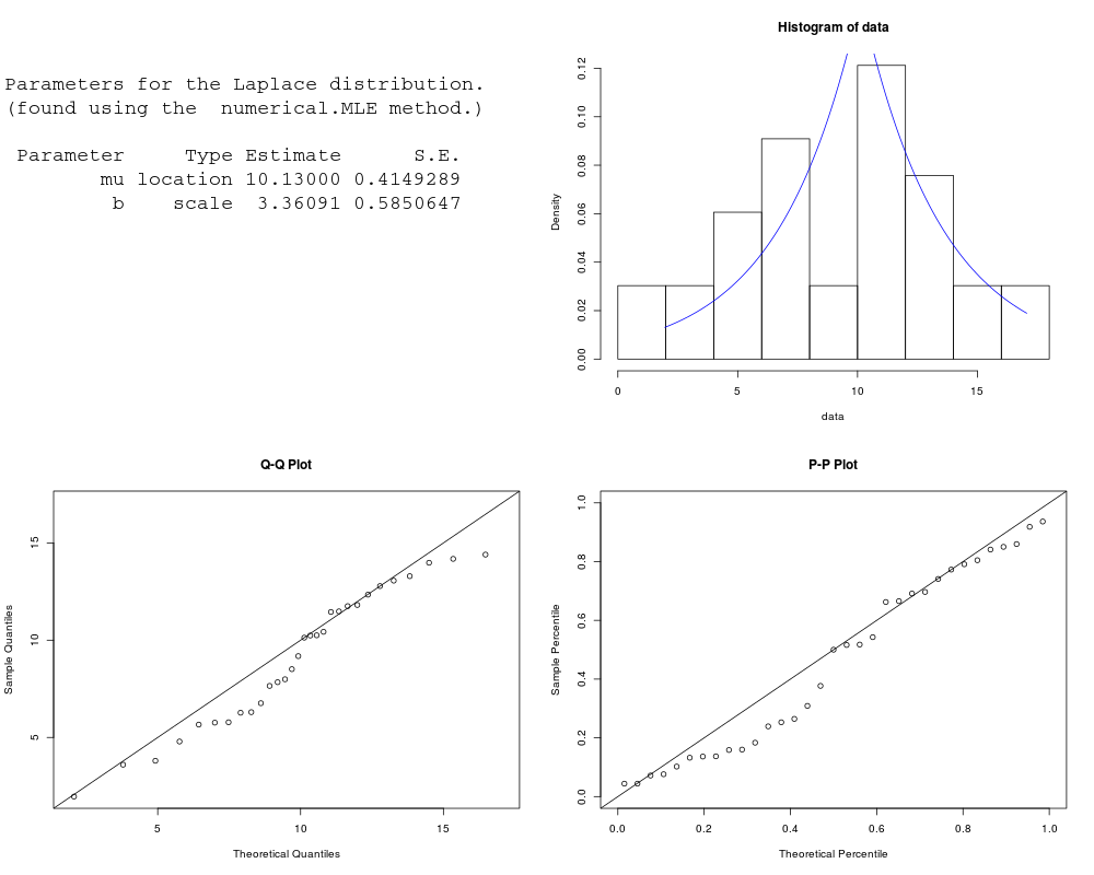
est.par <- eLaplace(flood, method="numerical.MLE"); est.par
plot(est.par)

#log-likelihood function
lLaplace(flood,param=est.par)

# Evaluating the precision by the Hessian matrix
H <- attributes(est.par)$nll.hessian
var <- solve(H)
se <- sqrt(diag(var));se

Results

R version 3.3.1 (2016-06-21) -- "Bug in Your Hair"
Copyright (C) 2016 The R Foundation for Statistical Computing
Platform: x86_64-pc-linux-gnu (64-bit)

R is free software and comes with ABSOLUTELY NO WARRANTY.
You are welcome to redistribute it under certain conditions.
Type 'license()' or 'licence()' for distribution details.

R is a collaborative project with many contributors.
Type 'contributors()' for more information and
'citation()' on how to cite R or R packages in publications.

Type 'demo()' for some demos, 'help()' for on-line help, or
'help.start()' for an HTML browser interface to help.
Type 'q()' to quit R.

> library(ExtDist)

Attaching package: 'ExtDist'

The following object is masked from 'package:stats':

    BIC

> png(filename="/home/ddbj/snapshot/RGM3/R_CC/result/ExtDist/Laplace.Rd_%03d_medium.png", width=480, height=480)
> ### Name: Laplace
> ### Title: The Laplace Distribution.
> ### Aliases: Laplace dLaplace eLaplace lLaplace pLaplace qLaplace rLaplace
> 
> ### ** Examples
> 
> # Parameter estimation for a distribution with known shape parameters
> X <- rLaplace(n=500, mu=1, b=2)
> est.par <- eLaplace(X, method="analytic.MLE"); est.par

Parameters for the Laplace distribution. 
(found using the  analytic.MLE method.)

 Parameter     Type  Estimate
        mu location 0.9297968
         b    scale 2.1685142


> plot(est.par)
> 
> #  Fitted density curve and histogram
> den.x <- seq(min(X),max(X),length=100)
> den.y <- dLaplace(den.x, location = est.par$location, scale= est.par$scale)
> hist(X, breaks=10, probability=TRUE, ylim = c(0,1.1*max(den.y)))
> lines(den.x, den.y, col="blue")
> lines(density(X), lty=2)
> 
> # Extracting location or scale parameters
> est.par[attributes(est.par)$par.type=="location"]
$mu
[1] 0.9297968

> est.par[attributes(est.par)$par.type=="scale"]
$b
[1] 2.168514

> 
> # Parameter estimation for a distribution with unknown shape parameters
> # Example from Best et.al (2008). Original source of flood data from Gumbel & Mustafi.
> # Parameter estimates as given by Best et.al mu=10.13 and  b=3.36
> flood <- c(1.96, 1.96, 3.60, 3.80, 4.79, 5.66, 5.76, 5.78, 6.27, 6.30, 6.76, 7.65, 7.84, 7.99,
+            8.51, 9.18, 10.13, 10.24, 10.25, 10.43, 11.45, 11.48, 11.75, 11.81, 12.34, 12.78, 13.06,
+            13.29, 13.98, 14.18, 14.40, 16.22, 17.06)
> est.par <- eLaplace(flood, method="numerical.MLE"); est.par

Parameters for the Laplace distribution. 
(found using the  numerical.MLE method.)

 Parameter     Type Estimate      S.E.
        mu location 10.13000 0.4149289
         b    scale  3.36091 0.5850647


> plot(est.par)
> 
> #log-likelihood function
> lLaplace(flood,param=est.par)
[1] -95.87684
> 
> # Evaluating the precision by the Hessian matrix
> H <- attributes(est.par)$nll.hessian
> var <- solve(H)
> se <- sqrt(diag(var));se
       mu         b 
0.4149289 0.5850647 
> 
> 
> 
> 
> 
> dev.off()
null device 
          1 
>