The Normal Distribution.

Description

Density, distribution, quantile, random number generation and parameter estimation functions for the normal distribution. Parameter estimation can be based on a weighted or unweighted i.i.d. sample and can be carried out analytically or numerically.

Usage

dNormal(x, mean = 0, sd = 1, params = list(mean, sd), ...)

pNormal(q, mean = 0, sd = 1, params = list(mean, sd), ...)

qNormal(p, mean = 0, sd = 1, params = list(mean, sd), ...)

rNormal(n, mean = 0, sd = 1, params = list(mean, sd), ...)

eNormal(X, w, method = c("unbiased.MLE", "analytical.MLE", "numerical.MLE"),
  ...)

lNormal(X, w, mean = 0, sd = 1, params = list(mean, sd), logL = TRUE,
  ...)

sNormal(X, w, mean = 0, sd = 1, params = list(mean, sd), ...)

iNormal(X, w, mean = 0, sd = 1, params = list(mean, sd), ...)

Arguments

Details

If the mean or sd are not specified they assume the default values of 0 and 1, respectively.

The dNormal(), pNormal(), qNormal(),and rNormal() functions serve as wrappers of the standard dnorm, pnorm, qnorm, and rnorm functions in the stats package. They allow for the parameters to be declared not only as individual numerical values, but also as a list so parameter estimation can be carried out.

The normal distribution has probability density function

f(x) = frac{1}{√{2 π} σ} e^{-frac{(x-μ)^2}{2σ^2}}

where μ is the mean of the distribution and σ is the standard deviation. The analytical unbiased parameter estimations are as given by Johnson et.al (Vol 1, pp.123-128).

The log-likelihood function of the normal distribution is given by

l(μ, σ| x) = ∑_{i}[-0.5 ln(2π) - ln(σ) - 0.5σ^{-2}(x_i-μ)^2].

The score function and observed information matrix are as given by Casella & Berger (2nd Ed, pp.321-322).

Value

dNormal gives the density, pNormal gives the distribution function, qNormal gives the quantiles, rNormal generates random deviates, and eNormal estimates the parameters. lNormal provides the log-likelihood function, sNormal the score function, and iNormal the observed information matrix.

Author(s)

Haizhen Wu and A. Jonathan R. Godfrey.
Updates and bug fixes by Sarah Pirikahu.

References

Johnson, N. L., Kotz, S. and Balakrishnan, N. (1994) Continuous Univariate Distributions, volume 1, chapter 13, Wiley, New York.

Casella, G. and Berger R. L. (2002) Statistical Inference, 2nd Ed, pp.321-322, Duxbury.

Bury, K. (1999) Statistical Distributions in Engineering, Chapter 10, p.143, Cambridge University Press.

See Also

ExtDist for other standard distributions.

Examples

# Parameter estimation for a distribution with known shape parameters
x <- rNormal(n=500, params=list(mean=1, sd=2))
est.par <- eNormal(X=x, method="unbiased.MLE"); est.par
plot(est.par)

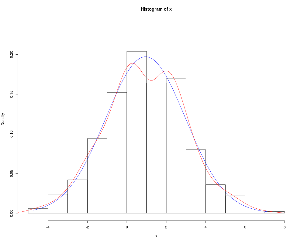
#  Fitted density curve and histogram
den.x <- seq(min(x),max(x),length=100)
den.y <- dNormal(den.x, mean = est.par$mean, sd = est.par$sd)
hist(x, breaks=10, probability=TRUE, ylim = c(0,1.2*max(den.y)))
lines(lines(den.x, den.y, col="blue")) # Original data
lines(density(x), col="red")           # Fitted curve

# Extracting location and scale parameters
est.par[attributes(est.par)$par.type=="location"]
est.par[attributes(est.par)$par.type=="scale"]

# Parameter Estimation for a distribution with unknown shape parameters
# Example from: Bury(1999) p.143, parameter estimates as given by Bury are
# mu = 11.984 and sigma = 0.067
data <- c(12.065, 11.992, 11.992, 11.921, 11.954, 11.945, 12.029, 11.948, 11.885, 11.997,
         11.982, 12.109, 11.966, 12.081, 11.846, 12.007, 12.011)
est.par <- eNormal(X=data, method="numerical.MLE"); est.par
plot(est.par)

# log-likelihood, score function and observed information matrix
lNormal(data, param = est.par)
sNormal(data, param = est.par)
iNormal(data, param = est.par)

# Evaluating the precision of the parameter estimates by the Hessian matrix
H <- attributes(est.par)$nll.hessian; H
var <- solve(H)
se <- sqrt(diag(var)); se

Results

R version 3.3.1 (2016-06-21) -- "Bug in Your Hair"
Copyright (C) 2016 The R Foundation for Statistical Computing
Platform: x86_64-pc-linux-gnu (64-bit)

R is free software and comes with ABSOLUTELY NO WARRANTY.
You are welcome to redistribute it under certain conditions.
Type 'license()' or 'licence()' for distribution details.

R is a collaborative project with many contributors.
Type 'contributors()' for more information and
'citation()' on how to cite R or R packages in publications.

Type 'demo()' for some demos, 'help()' for on-line help, or
'help.start()' for an HTML browser interface to help.
Type 'q()' to quit R.

> library(ExtDist)

Attaching package: 'ExtDist'

The following object is masked from 'package:stats':

    BIC

> png(filename="/home/ddbj/snapshot/RGM3/R_CC/result/ExtDist/Normal.Rd_%03d_medium.png", width=480, height=480)
> ### Name: Normal
> ### Title: The Normal Distribution.
> ### Aliases: Normal dNormal eNormal iNormal lNormal pNormal qNormal rNormal
> ###   sNormal
> 
> ### ** Examples
> 
> # Parameter estimation for a distribution with known shape parameters
> x <- rNormal(n=500, params=list(mean=1, sd=2))
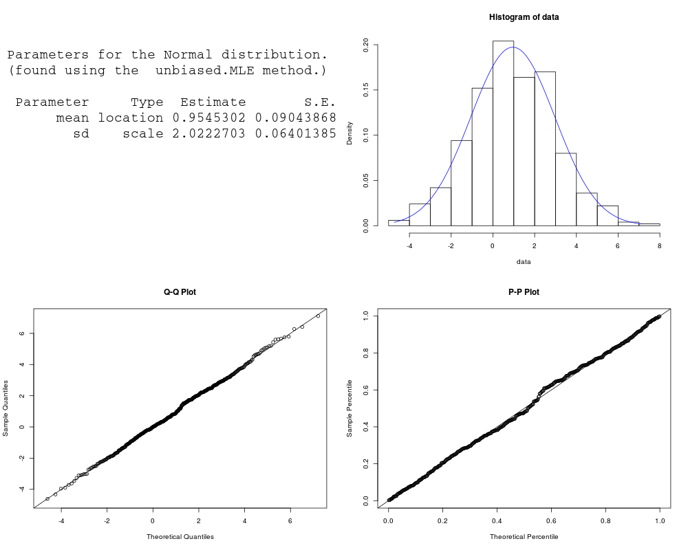
> est.par <- eNormal(X=x, method="unbiased.MLE"); est.par

Parameters for the Normal distribution. 
(found using the  unbiased.MLE method.)

 Parameter     Type  Estimate       S.E.
      mean location 0.9729552 0.09121550
        sd    scale 2.0396405 0.06456369


> plot(est.par)
> 
> #  Fitted density curve and histogram
> den.x <- seq(min(x),max(x),length=100)
> den.y <- dNormal(den.x, mean = est.par$mean, sd = est.par$sd)
> hist(x, breaks=10, probability=TRUE, ylim = c(0,1.2*max(den.y)))
> lines(lines(den.x, den.y, col="blue")) # Original data
> lines(density(x), col="red")           # Fitted curve
> 
> # Extracting location and scale parameters
> est.par[attributes(est.par)$par.type=="location"]
$mean
[1] 0.9729552

> est.par[attributes(est.par)$par.type=="scale"]
$sd
[1] 2.03964

> 
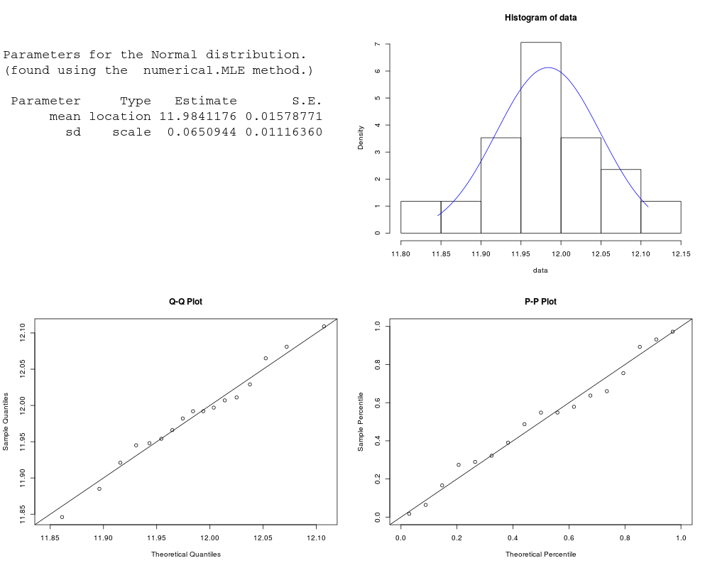
> # Parameter Estimation for a distribution with unknown shape parameters
> # Example from: Bury(1999) p.143, parameter estimates as given by Bury are
> # mu = 11.984 and sigma = 0.067
> data <- c(12.065, 11.992, 11.992, 11.921, 11.954, 11.945, 12.029, 11.948, 11.885, 11.997,
+          11.982, 12.109, 11.966, 12.081, 11.846, 12.007, 12.011)
> est.par <- eNormal(X=data, method="numerical.MLE"); est.par

Parameters for the Normal distribution. 
(found using the  numerical.MLE method.)

 Parameter     Type   Estimate       S.E.
      mean location 11.9841176 0.01578771
        sd    scale  0.0650944 0.01116360


> plot(est.par)
> 
> # log-likelihood, score function and observed information matrix
> lNormal(data, param = est.par)
[1] 22.32063
> sNormal(data, param = est.par)
         mean            sd 
 4.051759e-06 -1.505957e-05 
> iNormal(data, param = est.par)
             mean           sd
mean 4.012007e+03 1.244887e-04
sd   1.244887e-04 8.024014e+03
> 
> # Evaluating the precision of the parameter estimates by the Hessian matrix
> H <- attributes(est.par)$nll.hessian; H
             mean           sd
mean 4.012007e+03 1.244887e-04
sd   1.244887e-04 8.024014e+03
> var <- solve(H)
> se <- sqrt(diag(var)); se
      mean         sd 
0.01578771 0.01116360 
> 
> 
> 
> 
> 
> dev.off()
null device 
          1 
>