Supported by Dr. Osamu Ogasawara and  . . |
|
Last data update: 2014.03.03 |
Framework for Modeling Interactions with Strong HeredityDescriptionThis function runs the main algorithm presented in Haris, Witten and Simon (2014) for fitting an interaction model with strong heredity. Usage
FAMILY(X, Z, Y, lambdas , alphas, family = c("gaussian","binomial"),
    rho = 1, B = NULL, norm = "l2", quad = TRUE,iter=500,
    e.abs = 1e-3, e.rel = 1e-3,
    maxiter.B = 50, tol.B = 1e-04, verbose = FALSE)
Arguments
DetailsThis function fits a regression model based with pair-wise interaction terms by solving the optimization problem (33)(linear regression) or (35)(logistic regression) in Haris, Witten and Simon (2014). The optimization problem is solved via an ADMM algorithm. ValueThe function returns a list where the first component,
The function also returns the training data used to fit the model and the path of penalty parameters for which we estimated the model. ReferencesHaris, Witten and Simon (2014). Convex Modeling of Interactions with Strong Heredity. Available on ArXiv at http://arxiv.org/abs/1410.3517. Boyd, Stephen, et al. "Distributed optimization and statistical learning via the alternating direction method of multipliers." Foundations and Trends? in Machine Learning 3.1 (2011): 1-122. See Also
Examples
library(FAMILY)
library(pROC)
library(pheatmap)
#####################################################################################
#####################################################################################
############################# EXAMPLE - CONTINUOUS RESPONSE #########################
#####################################################################################
#####################################################################################
############################## GENERATE DATA ########################################
#Generate training set of covariates X and Z
set.seed(1)
X.tr<- matrix(rnorm(10*100),ncol = 10, nrow = 100)
Z.tr<- matrix(rnorm(15*100),ncol = 15, nrow = 100)
#Generate test set of covariates X and Z
X.te<- matrix(rnorm(10*100),ncol = 10, nrow = 100)
Z.te<- matrix(rnorm(15*100),ncol = 15, nrow = 100)
#Scale appropiately
meanX<- apply(X.tr,2,mean)
meanY<- apply(Z.tr,2,mean)
X.tr<- scale(X.tr, scale = FALSE)
Z.tr<- scale(Z.tr, scale = FALSE)
X.te<- scale(X.te,center = meanX,scale = FALSE)
Z.te<- scale(Z.te,center = meanY,scale = FALSE)
#Generate full matrix of Covariates
w.tr<- c()
w.te<- c()
X1<- cbind(1,X.tr)
Z1<- cbind(1,Z.tr)
X2<- cbind(1,X.te)
Z2<- cbind(1,Z.te)
for(i in 1:16){
for(j in 1:11){
w.tr<- cbind(w.tr,X1[,j]*Z1[,i])
w.te<- cbind(w.te, X2[,j]*Z2[,i])
}
}
#Generate response variables with signal from
#First 5 X features and 5 Z features.
#We construct the coefficient matrix B.
#B[1,1] contains the intercept
#B[-1,1] contains the main effects for X.
# For instance, B[2,1] is the main effect for the first feature in X.
#B[1,-1] contains the main effects for Z.
# For instance, B[1,10] is the coefficient for the 10th feature in Z.
#B[i+1,j+1] is the coefficient of X_i Z_j
B<- matrix(0,ncol = 16,nrow = 11)
rownames(B)<- c("inter" , paste("X",1:(nrow(B)-1),sep = ""))
colnames(B)<- c("inter" , paste("Z",1:(ncol(B)-1),sep = ""))
# First, we simulate data as follows:
# The first five features in X, and the first five features in Z, are non-zero.
# And given the non-zero main effects, all possible interactions are involved.
# We call this "high strong heredity"
B_high_SH<- B
B_high_SH[1:6,1:6]<- 1
#View true coefficient matrix
pheatmap(as.matrix(B_high_SH), scale="none",
cluster_rows=FALSE, cluster_cols=FALSE)
Y_high_SH <- as.vector(w.tr%*%as.vector(B_high_SH))+rnorm(100,sd = 2)
Y_high_SH.te <- as.vector(w.te%*%as.vector(B_high_SH))+rnorm(100,sd = 2)
# Now a new setting:
# Again, the first five features in X, and the first five features in Z, are involved.
# But this time, only a subset of the possible interactions are involved.
# Strong heredity is still maintained.
# We call this "low strong heredity"
B_low_SH<- B_high_SH
B_low_SH[2:6,2:6]<-0
B_low_SH[3:4,3:5]<- 1
#View true coefficient matrix
pheatmap(as.matrix(B_low_SH), scale="none",
cluster_rows=FALSE, cluster_cols=FALSE)
Y_low_SH <- as.vector(w.tr%*%as.vector(B_low_SH))+rnorm(100,sd = 1.5)
Y_low_SH.te <- as.vector(w.te%*%as.vector(B_low_SH))+rnorm(100,sd = 1.5)
############################## FIT SOME MODELS ########################################
#Define alphas and lambdas
#Define 3 different alpha values
#Low alpha values penalize groups more
#High alpha values penalize individual Interactions more
alphas<- c(0.01,0.5,0.99)
lambdas<- seq(0.1,1,length = 50)
#high Strong heredity with l2 norm
fit_high_SH<- FAMILY(X.tr, Z.tr, Y_high_SH, lambdas ,
alphas, quad = TRUE,iter=500, verbose = TRUE )
yhat_hSH<- predict(fit_high_SH, X.te, Z.te)
mse_hSH <-apply(yhat_hSH,c(2,3), "-" ,Y_high_SH.te)
mse_hSH<- apply(mse_hSH^2,c(2,3),sum)
#Find optimal model and plot matrix
im<- which(mse_hSH==min(mse_hSH),TRUE)
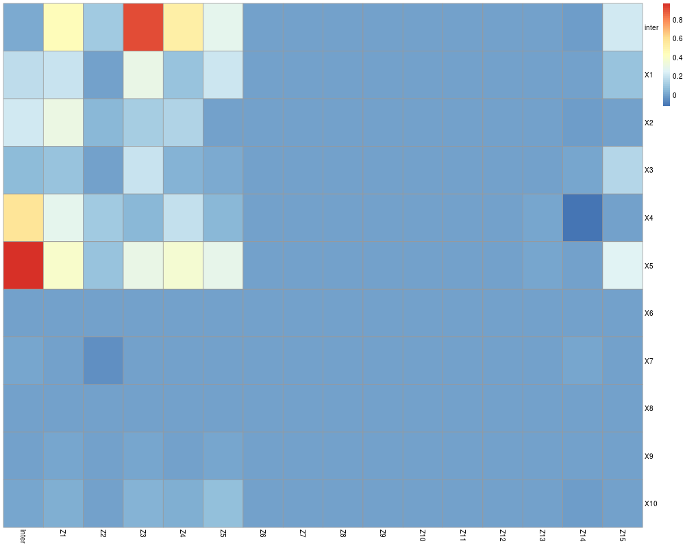
plot(fit_high_SH$Estimate[[im[2] ]][[im[1]]])
#Plot some matrices for different alpha values
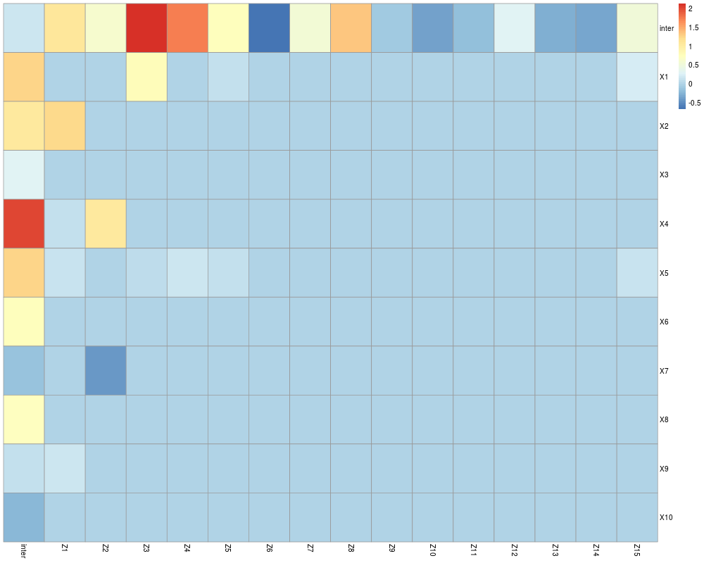
#Low alpha, higher penalty on groups
plot(fit_high_SH$Estimate[[ 1 ]][[ 25 ]])
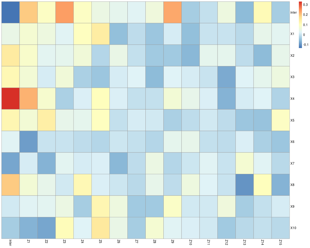
#Medium alpha, equal penalty on groups and individual interactions
plot(fit_high_SH$Estimate[[ 2 ]][[ 25 ]])
#High alpha, more penalty on individual interactions
plot(fit_high_SH$Estimate[[ 3 ]][[ 40 ]])
#View Coefficients
coef(fit_high_SH)[[im[2]]][[im[1]]]
############################## Uncomment code for EXAMPLE ###########################
# #high Strong heredity with l_infinity norm norm
# fit_high_SH<- FAMILY(X.tr, Z.tr, Y_high_SH, lambdas ,
# alphas, quad = TRUE,iter=500, verbose = TRUE,
# norm = "l_inf")
# yhat_hSH<- predict(fit_high_SH, X.te, Z.te)
# mse_hSH <-apply(yhat_hSH,c(2,3), "-" ,Y_high_SH.te)
# mse_hSH<- apply(mse_hSH^2,c(2,3),sum)
#
# #Find optimal model and plot matrix
# im<- which(mse_hSH==min(mse_hSH),TRUE)
# plot(fit_high_SH$Estimate[[im[2] ]][[im[1]]])
#
#
# #Plot some matrices for different alpha values
# #Low alpha, higher penalty on groups
# plot(fit_high_SH$Estimate[[ 1 ]][[ 30 ]])
# #Medium alpha, equal penalty on groups and individual interactions
# plot(fit_high_SH$Estimate[[ 2 ]][[ 10 ]])
# #High alpha, more penalty on individual interactions
# plot(fit_high_SH$Estimate[[ 3 ]][[ 20 ]])
#
#
# #View Coefficients
# coef(fit_high_SH)[[im[2]]][[im[1]]]
############################## Uncomment code for EXAMPLE ###########################
# #Redefine lambdas
# lambdas<- seq(0.1,0.5,length = 50)
#
# #low Strong heredity with l_2 norm
# fit_low_SH<- FAMILY(X.tr, Z.tr, Y_low_SH, lambdas ,
# alphas, quad = TRUE,iter=500, verbose = TRUE )
# yhat_lSH<- predict(fit_low_SH, X.te, Z.te)
# mse_lSH <-apply(yhat_lSH,c(2,3), "-" ,Y_low_SH.te)
# mse_lSH<- apply(mse_lSH^2,c(2,3),sum)
#
# #Find optimal model and plot matrix
# im<- which(mse_lSH==min(mse_lSH),TRUE)
# plot(fit_low_SH$Estimate[[im[2] ]][[im[1]]])
#
#
# #Plot some matrices for different alpha values
# #Low alpha, higher penalty on groups
# plot(fit_low_SH$Estimate[[ 1 ]][[ 25 ]])
# #Medium alpha, equal penalty on groups and individual interactions
# plot(fit_low_SH$Estimate[[ 2 ]][[ 10 ]])
# #High alpha, more penalty on individual interactions
# plot(fit_low_SH$Estimate[[ 3 ]][[ 10 ]])
#
#
# #View Coefficients
# coef(fit_low_SH)[[im[2]]][[im[1]]]
#####################################################################################
#####################################################################################
############################### EXAMPLE - BINARY RESPONSE ###########################
#####################################################################################
#####################################################################################
############################## GENERATE DATA ########################################
#Generate data for logistic regression
Yp_high_SH<- as.vector((w.tr)%*%as.vector(B_high_SH))
Yp_high_SH.te<- as.vector((w.te)%*%as.vector(B_high_SH))
Yprobs_high_SH<- 1/(1+exp(-Yp_high_SH))
Yprobs_high_SH.te<- 1/(1+exp(-Yp_high_SH.te))
Yp_high_SH<- rbinom(100, size = 1, prob = Yprobs_high_SH)
Yp_high_SH.te<- rbinom(100, size = 1, prob = Yprobs_high_SH.te)
lambdas<- seq(0.01,0.15,length = 50)
############################## FIT SOME MODELS ########################################
#Fit glm via l_2 norm
fit_high_SH<- FAMILY(X.tr, Z.tr, Yp_high_SH, lambdas ,
alphas, quad = TRUE,iter=500, verbose = TRUE,
family = "binomial")
yhp_hSH<- predict(fit_high_SH, X.te, Z.te)
mse_high_SH <-apply(yhp_hSH,c(2,3), "-" ,Yp_high_SH.te)
mse_hSH<- apply(mse_high_SH^2,c(2,3),sum)
im<- which(mse_hSH==min(mse_hSH),TRUE)
plot(fit_high_SH$Estimate[[im[2] ]][[im[1]]])
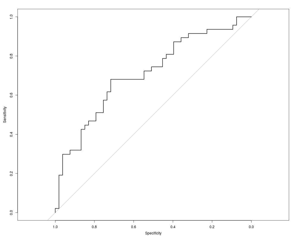
roc( Yp_high_SH.te,yhp_hSH[,im[1],im[2]],plot = TRUE)
#View Coefficients
coef(fit_high_SH)[[im[2]]][[im[1]]]
############################## Uncomment code for EXAMPLE ###########################
# #Fit glm via l_infinity norm
# fit_high_SH<- FAMILY(X.tr, Z.tr, Yp_high_SH, lambdas , norm = "l_inf",
# alphas, quad = TRUE,iter=500, verbose = TRUE,
# family = "binomial")
# yhp_hSH<- predict(fit_high_SH, X.te, Z.te)
# mse_high_SH <-apply(yhp_hSH,c(2,3), "-" ,Yp_high_SH.te)
# mse_hSH<- apply(mse_high_SH^2,c(2,3),sum)
# im<- which(mse_hSH==min(mse_hSH),TRUE)
# plot(fit_high_SH$Estimate[[im[2] ]][[im[1]]])
# roc( Yp_high_SH.te,yhp_hSH[,im[1],im[2]],plot = TRUE)
#
# #View Coefficients
# coef(fit_high_SH)[[im[2]]][[im[1]]]
#####################################################################################
#####################################################################################
############################## EXAMPLE WHERE X=Z ####################################
######################## Uncomment Code for EXAMPLE #################################
#####################################################################################
############################## GENERATE DATA ########################################
# #Redefine Lambdas
# lambdas<- seq(0.01,0.3,length = 50)
#
#
# #We consider the case X=Z now
# w.tr<- c()
# w.te<- c()
# X1<- cbind(1,X.tr)
# X2<- cbind(1,X.te)
#
# for(i in 1:11){
# for(j in 1:11){
# w.tr<- cbind(w.tr,X1[,j]*X1[,i])
# w.te<- cbind(w.te, X2[,j]*X2[,i])
# }
# }
#
# B<- matrix(0,ncol = 11,nrow = 11)
# rownames(B)<- c("inter" , paste("X",1:(nrow(B)-1),sep = ""))
# colnames(B)<- c("inter" , paste("X",1:(ncol(B)-1),sep = ""))
#
#
# B_high_SH<- B
# B_high_SH[1:6,1:6]<- 1
# #We exclude quadratic terms in this example
# diag(B_high_SH)[-1]<-0
# #View true coefficient matrix
# pheatmap(as.matrix(B_high_SH), scale="none",
# cluster_rows=FALSE, cluster_cols=FALSE)
#
# #With high Strong heredity: all possible interactions
# Y_high_SH <- as.vector(w.tr%*%as.vector(B_high_SH))+rnorm(100)
# Y_high_SH.te <- as.vector(w.te%*%as.vector(B_high_SH))+rnorm(100)
#
# ############################## FIT SOME MODELS ########################################
#
# #high Strong heredity with l_2 norm
# fit_high_SH<- FAMILY(X.tr, X.tr, Y_high_SH, lambdas ,
# alphas, quad = FALSE,iter=500, verbose = TRUE )
# yhat_hSH<- predict(fit_high_SH, X.te, X.te)
# mse_hSH <-apply(yhat_hSH,c(2,3), "-" ,Y_high_SH.te)
# mse_hSH<- apply(mse_hSH^2,c(2,3),sum)
#
# #Find optimal model and plot matrix
# im<- which(mse_hSH==min(mse_hSH),TRUE)
# plot(fit_high_SH$Estimate[[im[2] ]][[im[1]]])
#
#
# #Plot some matrices for different alpha values
# #Low alpha, higher penalty on groups
# plot(fit_high_SH$Estimate[[ 1 ]][[ 50 ]])
# #Medium alpha, equal penalty on groups and individual interactions
# plot(fit_high_SH$Estimate[[ 2 ]][[ 50 ]])
# #High alpha, more penalty on individual interactions
# plot(fit_high_SH$Estimate[[ 3 ]][[ 50 ]])
#
#
# #View Coefficients
# coef(fit_high_SH,XequalZ = TRUE)[[im[2]]][[im[1]]]
Results
R version 3.3.1 (2016-06-21) -- "Bug in Your Hair"
Copyright (C) 2016 The R Foundation for Statistical Computing
Platform: x86_64-pc-linux-gnu (64-bit)

R is free software and comes with ABSOLUTELY NO WARRANTY.
You are welcome to redistribute it under certain conditions.
Type 'license()' or 'licence()' for distribution details.

R is a collaborative project with many contributors.
Type 'contributors()' for more information and
'citation()' on how to cite R or R packages in publications.

Type 'demo()' for some demos, 'help()' for on-line help, or
'help.start()' for an HTML browser interface to help.
Type 'q()' to quit R.

> library(FAMILY)
> png(filename="/home/ddbj/snapshot/RGM3/R_CC/result/FAMILY/FAMILY.Rd_%03d_medium.png", width=480, height=480)
> ### Name: FAMILY
> ### Title: Framework for Modeling Interactions with Strong Heredity
> ### Aliases: FAMILY
>
> ### ** Examples
>
> library(FAMILY)
> library(pROC)
Type 'citation("pROC")' for a citation.

Attaching package: 'pROC'

The following objects are masked from 'package:stats':

    cov, smooth, var

> library(pheatmap)
>
> #####################################################################################
> #####################################################################################
> ############################# EXAMPLE - CONTINUOUS RESPONSE #########################
> #####################################################################################
> #####################################################################################
>
> ############################## GENERATE DATA ########################################
>
> #Generate training set of covariates X and Z
> set.seed(1)
> X.tr<- matrix(rnorm(10*100),ncol = 10, nrow = 100)
> Z.tr<- matrix(rnorm(15*100),ncol = 15, nrow = 100)
>
>
> #Generate test set of covariates X and Z
> X.te<- matrix(rnorm(10*100),ncol = 10, nrow = 100)
> Z.te<- matrix(rnorm(15*100),ncol = 15, nrow = 100)
>
> #Scale appropiately
> meanX<- apply(X.tr,2,mean)
> meanY<- apply(Z.tr,2,mean)
>
> X.tr<- scale(X.tr, scale = FALSE)
> Z.tr<- scale(Z.tr, scale = FALSE)
> X.te<- scale(X.te,center = meanX,scale = FALSE)
> Z.te<- scale(Z.te,center = meanY,scale = FALSE)
>
> #Generate full matrix of Covariates
> w.tr<- c()
> w.te<- c()
> X1<- cbind(1,X.tr)
> Z1<- cbind(1,Z.tr)
> X2<- cbind(1,X.te)
> Z2<- cbind(1,Z.te)
>
> for(i in 1:16){
+   for(j in 1:11){
+     w.tr<- cbind(w.tr,X1[,j]*Z1[,i])
+     w.te<- cbind(w.te, X2[,j]*Z2[,i])
+   }
+ }
>
> #Generate response variables with signal from
> #First 5 X features and 5 Z features.
>
> #We construct the coefficient matrix B.
> #B[1,1] contains the intercept
> #B[-1,1] contains the main effects for X.
> # For instance, B[2,1] is the main effect for the first feature in X.
> #B[1,-1] contains the main effects for Z.
> # For instance, B[1,10] is the coefficient for the 10th feature in Z.
> #B[i+1,j+1] is the coefficient of X_i Z_j
> B<- matrix(0,ncol = 16,nrow = 11)
> rownames(B)<- c("inter" , paste("X",1:(nrow(B)-1),sep = ""))
> colnames(B)<- c("inter" , paste("Z",1:(ncol(B)-1),sep = ""))
>
> # First, we simulate data as follows:
> # The first five features in X, and the first five features in Z, are non-zero.
> # And given the non-zero main effects, all possible interactions are involved.
> # We call this "high strong heredity"
> B_high_SH<- B
> B_high_SH[1:6,1:6]<- 1
> #View true coefficient matrix
> pheatmap(as.matrix(B_high_SH), scale="none",
+          cluster_rows=FALSE, cluster_cols=FALSE)
>
> Y_high_SH <- as.vector(w.tr%*%as.vector(B_high_SH))+rnorm(100,sd = 2)
> Y_high_SH.te <- as.vector(w.te%*%as.vector(B_high_SH))+rnorm(100,sd = 2)
>
> # Now a new setting:
> # Again, the first five features in X, and the first five features in Z, are involved.
> # But this time, only a subset of the possible interactions are involved.
> # Strong heredity is still maintained.
> # We call this "low strong heredity"
> B_low_SH<- B_high_SH
> B_low_SH[2:6,2:6]<-0
> B_low_SH[3:4,3:5]<- 1
> #View true coefficient matrix
> pheatmap(as.matrix(B_low_SH), scale="none",
+          cluster_rows=FALSE, cluster_cols=FALSE)
> Y_low_SH <- as.vector(w.tr%*%as.vector(B_low_SH))+rnorm(100,sd = 1.5)
> Y_low_SH.te <- as.vector(w.te%*%as.vector(B_low_SH))+rnorm(100,sd = 1.5)
>
>
> ############################## FIT SOME MODELS ########################################
>
> #Define alphas and lambdas
> #Define 3 different alpha values
> #Low alpha values penalize groups more
> #High alpha values penalize individual Interactions more
> alphas<- c(0.01,0.5,0.99)
> lambdas<- seq(0.1,1,length = 50)
>
> #high Strong heredity with l2 norm
> fit_high_SH<- FAMILY(X.tr, Z.tr, Y_high_SH, lambdas ,
+                      alphas, quad = TRUE,iter=500, verbose = TRUE )
Computing w...done.
Starting svd...done.
Fitting model for alpha = 0.01 and lambda = 1
Fitting model for alpha = 0.01 and lambda = 0.98
Fitting model for alpha = 0.01 and lambda = 0.96
Fitting model for alpha = 0.01 and lambda = 0.94
Fitting model for alpha = 0.01 and lambda = 0.93
Fitting model for alpha = 0.01 and lambda = 0.91
Fitting model for alpha = 0.01 and lambda = 0.89
Fitting model for alpha = 0.01 and lambda = 0.87
Fitting model for alpha = 0.01 and lambda = 0.85
Fitting model for alpha = 0.01 and lambda = 0.83
Fitting model for alpha = 0.01 and lambda = 0.82
Fitting model for alpha = 0.01 and lambda = 0.8
Fitting model for alpha = 0.01 and lambda = 0.78
Fitting model for alpha = 0.01 and lambda = 0.76
Fitting model for alpha = 0.01 and lambda = 0.74
Fitting model for alpha = 0.01 and lambda = 0.72
Fitting model for alpha = 0.01 and lambda = 0.71
Fitting model for alpha = 0.01 and lambda = 0.69
Fitting model for alpha = 0.01 and lambda = 0.67
Fitting model for alpha = 0.01 and lambda = 0.65
Fitting model for alpha = 0.01 and lambda = 0.63
Fitting model for alpha = 0.01 and lambda = 0.61
Fitting model for alpha = 0.01 and lambda = 0.6
Fitting model for alpha = 0.01 and lambda = 0.58
Fitting model for alpha = 0.01 and lambda = 0.56
Fitting model for alpha = 0.01 and lambda = 0.54
Fitting model for alpha = 0.01 and lambda = 0.52
Fitting model for alpha = 0.01 and lambda = 0.5
Fitting model for alpha = 0.01 and lambda = 0.49
Fitting model for alpha = 0.01 and lambda = 0.47
Fitting model for alpha = 0.01 and lambda = 0.45
Fitting model for alpha = 0.01 and lambda = 0.43
Fitting model for alpha = 0.01 and lambda = 0.41
Fitting model for alpha = 0.01 and lambda = 0.39
Fitting model for alpha = 0.01 and lambda = 0.38
Fitting model for alpha = 0.01 and lambda = 0.36
Fitting model for alpha = 0.01 and lambda = 0.34
Fitting model for alpha = 0.01 and lambda = 0.32
Fitting model for alpha = 0.01 and lambda = 0.3
Fitting model for alpha = 0.01 and lambda = 0.28
Fitting model for alpha = 0.01 and lambda = 0.27
Fitting model for alpha = 0.01 and lambda = 0.25
Fitting model for alpha = 0.01 and lambda = 0.23
Fitting model for alpha = 0.01 and lambda = 0.21
Fitting model for alpha = 0.01 and lambda = 0.19
Fitting model for alpha = 0.01 and lambda = 0.17
Fitting model for alpha = 0.01 and lambda = 0.16
Fitting model for alpha = 0.01 and lambda = 0.14
Fitting model for alpha = 0.01 and lambda = 0.12
Fitting model for alpha = 0.01 and lambda = 0.1
Fitting model for alpha = 0.5 and lambda = 1
Fitting model for alpha = 0.5 and lambda = 0.98
Fitting model for alpha = 0.5 and lambda = 0.96
Fitting model for alpha = 0.5 and lambda = 0.94
Fitting model for alpha = 0.5 and lambda = 0.93
Fitting model for alpha = 0.5 and lambda = 0.91
Fitting model for alpha = 0.5 and lambda = 0.89
Fitting model for alpha = 0.5 and lambda = 0.87
Fitting model for alpha = 0.5 and lambda = 0.85
Fitting model for alpha = 0.5 and lambda = 0.83
Fitting model for alpha = 0.5 and lambda = 0.82
Fitting model for alpha = 0.5 and lambda = 0.8
Fitting model for alpha = 0.5 and lambda = 0.78
Fitting model for alpha = 0.5 and lambda = 0.76
Fitting model for alpha = 0.5 and lambda = 0.74
Fitting model for alpha = 0.5 and lambda = 0.72
Fitting model for alpha = 0.5 and lambda = 0.71
Fitting model for alpha = 0.5 and lambda = 0.69
Fitting model for alpha = 0.5 and lambda = 0.67
Fitting model for alpha = 0.5 and lambda = 0.65
Fitting model for alpha = 0.5 and lambda = 0.63
Fitting model for alpha = 0.5 and lambda = 0.61
Fitting model for alpha = 0.5 and lambda = 0.6
Fitting model for alpha = 0.5 and lambda = 0.58
Fitting model for alpha = 0.5 and lambda = 0.56
Fitting model for alpha = 0.5 and lambda = 0.54
Fitting model for alpha = 0.5 and lambda = 0.52
Fitting model for alpha = 0.5 and lambda = 0.5
Fitting model for alpha = 0.5 and lambda = 0.49
Fitting model for alpha = 0.5 and lambda = 0.47
Fitting model for alpha = 0.5 and lambda = 0.45
Fitting model for alpha = 0.5 and lambda = 0.43
Fitting model for alpha = 0.5 and lambda = 0.41
Fitting model for alpha = 0.5 and lambda = 0.39
Fitting model for alpha = 0.5 and lambda = 0.38
Fitting model for alpha = 0.5 and lambda = 0.36
Fitting model for alpha = 0.5 and lambda = 0.34
Fitting model for alpha = 0.5 and lambda = 0.32
Fitting model for alpha = 0.5 and lambda = 0.3
Fitting model for alpha = 0.5 and lambda = 0.28
Fitting model for alpha = 0.5 and lambda = 0.27
Fitting model for alpha = 0.5 and lambda = 0.25
Fitting model for alpha = 0.5 and lambda = 0.23
Fitting model for alpha = 0.5 and lambda = 0.21
Fitting model for alpha = 0.5 and lambda = 0.19
Fitting model for alpha = 0.5 and lambda = 0.17
Fitting model for alpha = 0.5 and lambda = 0.16
Fitting model for alpha = 0.5 and lambda = 0.14
Fitting model for alpha = 0.5 and lambda = 0.12
Fitting model for alpha = 0.5 and lambda = 0.1
Fitting model for alpha = 0.99 and lambda = 1
Fitting model for alpha = 0.99 and lambda = 0.98
Fitting model for alpha = 0.99 and lambda = 0.96
Fitting model for alpha = 0.99 and lambda = 0.94
Fitting model for alpha = 0.99 and lambda = 0.93
Fitting model for alpha = 0.99 and lambda = 0.91
Fitting model for alpha = 0.99 and lambda = 0.89
Fitting model for alpha = 0.99 and lambda = 0.87
Fitting model for alpha = 0.99 and lambda = 0.85
Fitting model for alpha = 0.99 and lambda = 0.83
Fitting model for alpha = 0.99 and lambda = 0.82
Fitting model for alpha = 0.99 and lambda = 0.8
Fitting model for alpha = 0.99 and lambda = 0.78
Fitting model for alpha = 0.99 and lambda = 0.76
Fitting model for alpha = 0.99 and lambda = 0.74
Fitting model for alpha = 0.99 and lambda = 0.72
Fitting model for alpha = 0.99 and lambda = 0.71
Fitting model for alpha = 0.99 and lambda = 0.69
Fitting model for alpha = 0.99 and lambda = 0.67
Fitting model for alpha = 0.99 and lambda = 0.65
Fitting model for alpha = 0.99 and lambda = 0.63
Fitting model for alpha = 0.99 and lambda = 0.61
Fitting model for alpha = 0.99 and lambda = 0.6
Fitting model for alpha = 0.99 and lambda = 0.58
Fitting model for alpha = 0.99 and lambda = 0.56
Fitting model for alpha = 0.99 and lambda = 0.54
Fitting model for alpha = 0.99 and lambda = 0.52
Fitting model for alpha = 0.99 and lambda = 0.5
Fitting model for alpha = 0.99 and lambda = 0.49
Fitting model for alpha = 0.99 and lambda = 0.47
Fitting model for alpha = 0.99 and lambda = 0.45
Fitting model for alpha = 0.99 and lambda = 0.43
Fitting model for alpha = 0.99 and lambda = 0.41
Fitting model for alpha = 0.99 and lambda = 0.39
Fitting model for alpha = 0.99 and lambda = 0.38
Fitting model for alpha = 0.99 and lambda = 0.36
Fitting model for alpha = 0.99 and lambda = 0.34
Fitting model for alpha = 0.99 and lambda = 0.32
Fitting model for alpha = 0.99 and lambda = 0.3
Fitting model for alpha = 0.99 and lambda = 0.28
Fitting model for alpha = 0.99 and lambda = 0.27
Fitting model for alpha = 0.99 and lambda = 0.25
Fitting model for alpha = 0.99 and lambda = 0.23
Fitting model for alpha = 0.99 and lambda = 0.21
Fitting model for alpha = 0.99 and lambda = 0.19
Fitting model for alpha = 0.99 and lambda = 0.17
Fitting model for alpha = 0.99 and lambda = 0.16
Fitting model for alpha = 0.99 and lambda = 0.14
Fitting model for alpha = 0.99 and lambda = 0.12
Fitting model for alpha = 0.99 and lambda = 0.1
> yhat_hSH<- predict(fit_high_SH, X.te, Z.te)
> mse_hSH <-apply(yhat_hSH,c(2,3), "-" ,Y_high_SH.te)
> mse_hSH<- apply(mse_hSH^2,c(2,3),sum)
>
> #Find optimal model and plot matrix
> im<- which(mse_hSH==min(mse_hSH),TRUE)
> plot(fit_high_SH$Estimate[[im[2] ]][[im[1]]])
>
>
> #Plot some matrices for different alpha values
> #Low alpha, higher penalty on groups
> plot(fit_high_SH$Estimate[[ 1 ]][[ 25 ]])
> #Medium alpha, equal penalty on groups and individual interactions
> plot(fit_high_SH$Estimate[[ 2 ]][[ 25  ]])
> #High alpha, more penalty on individual interactions
> plot(fit_high_SH$Estimate[[ 3 ]][[ 40 ]])
>
>
> #View Coefficients
> coef(fit_high_SH)[[im[2]]][[im[1]]]
$intercept
[1] 0.3660612

$mainsX
       X   Coef. est
 [1,]  1  0.74106671
 [2,]  2  0.87199302
 [3,]  3  0.44399664
 [4,]  4  1.06040396
 [5,]  5  0.90672267
 [6,]  6  0.39625494
 [7,]  7  0.08497034
 [8,]  8  0.17097666
 [9,]  9  0.04380046
[10,] 10 -0.26754722

$mainsZ
       Z   Coef. est
 [1,]  1  1.08763353
 [2,]  2  0.58585423
 [3,]  3  1.17322318
 [4,]  4  1.49858095
 [5,]  5  0.45218668
 [6,]  6 -0.17905849
 [7,]  7  0.07041749
 [8,]  8  0.31521911
 [9,]  9  0.04037807
[10,] 10 -0.06547316
[11,] 11  0.01708619
[12,] 12  0.11525280
[13,] 13 -0.10127333
[14,] 14 -0.25104818
[15,] 15  0.36484388

$interacts
        X  Z     Coef. est
  [1,]  1  1  0.5578295369
  [2,]  1  2  0.1730776965
  [3,]  1  3  0.8148027338
  [4,]  1  4  0.5571329635
  [5,]  1  5  0.7319715830
  [6,]  1  9  0.0575240437
  [7,]  1 13 -0.0347470090
  [8,]  1 15  0.1352830738
  [9,]  2  1  0.9619192679
 [10,]  2  2  0.3812697455
 [11,]  2  3  0.5303171103
 [12,]  2  4  0.7044951294
 [13,]  2  5  0.2083509789
 [14,]  2  6 -0.0271647282
 [15,]  2  8 -0.0163162853
 [16,]  2 14 -0.2233279117
 [17,]  2 15  0.0354304026
 [18,]  3  1  0.3364459150
 [19,]  3  3  0.6234262574
 [20,]  3  4  0.4301907858
 [21,]  3  5  0.2967603764
 [22,]  3  7 -0.0063398846
 [23,]  3  9 -0.1018623556
 [24,]  3 10  0.0544570736
 [25,]  3 12 -0.1035004436
 [26,]  3 13 -0.1653631979
 [27,]  3 15  0.4524197637
 [28,]  4  1  0.7865778697
 [29,]  4  2  0.5745010741
 [30,]  4  3  0.2576428284
 [31,]  4  4  0.5772894419
 [32,]  4  5  0.1966229935
 [33,]  4  6  0.0490099525
 [34,]  4  7 -0.0135553939
 [35,]  4 10  0.0767587686
 [36,]  4 12 -0.1186453677
 [37,]  4 13  0.0914928341
 [38,]  4 14 -0.5885422895
 [39,]  4 15 -0.0235524446
 [40,]  5  1  0.7173233720
 [41,]  5  2  0.5292900401
 [42,]  5  3  0.3394433282
 [43,]  5  4  0.7866571189
 [44,]  5  5  0.7259235462
 [45,]  5  6  0.0880023988
 [46,]  5  8  0.1090425242
 [47,]  5  9  0.0156231092
 [48,]  5 10  0.0307094983
 [49,]  5 11 -0.2548323690
 [50,]  5 12  0.0523544449
 [51,]  5 13  0.0353087829
 [52,]  5 14  0.0024335982
 [53,]  5 15  0.3332361674
 [54,]  6  1 -0.2526241673
 [55,]  6  4 -0.0629255692
 [56,]  6  6 -0.0179481274
 [57,]  6  7  0.0287249272
 [58,]  6  8 -0.1330999551
 [59,]  6  9  0.0077355010
 [60,]  6 10  0.1117550753
 [61,]  6 11  0.0947307799
 [62,]  6 12  0.0028421409
 [63,]  6 14 -0.2384378878
 [64,]  6 15 -0.0007264793
 [65,]  7  2 -0.3106003880
 [66,]  7  4 -0.0554199954
 [67,]  7  5  0.0896980472
 [68,]  7  6 -0.0364820452
 [69,]  7  7 -0.0471205773
 [70,]  7  8 -0.0019636384
 [71,]  7  9 -0.0548747534
 [72,]  7 12  0.0661508313
 [73,]  7 13 -0.0116683197
 [74,]  7 15  0.0754463279
 [75,]  8  1  0.0328937497
 [76,]  8  2 -0.0606613635
 [77,]  8  4  0.0177122799
 [78,]  8  5  0.0427344484
 [79,]  8  6  0.0229845376
 [80,]  8  7 -0.0317311056
 [81,]  8  9  0.0216367355
 [82,]  8 10 -0.0377712252
 [83,]  8 11 -0.0279991791
 [84,]  8 12  0.0276992068
 [85,]  8 13  0.0073108762
 [86,]  8 14  0.1210525668
 [87,]  9  1  0.2356221557
 [88,]  9  2  0.0091461121
 [89,]  9  3  0.0858649836
 [90,]  9  4  0.1325265779
 [91,]  9  5  0.2519507402
 [92,]  9  6  0.0011115372
 [93,]  9  8  0.1833241708
 [94,]  9  9  0.0175746888
 [95,]  9 10 -0.0824571059
 [96,]  9 14  0.0474901846
 [97,]  9 15 -0.0537351686
 [98,] 10  1  0.1202347003
 [99,] 10  2 -0.0636558169
[100,] 10  3  0.0976124448
[101,] 10  4  0.1847614426
[102,] 10  5  0.1111048832
[103,] 10  6  0.0219800374
[104,] 10  7  0.0125828537
[105,] 10  8  0.0551034109
[106,] 10 10 -0.0508601343
[107,] 10 11 -0.1371672610
[108,] 10 12 -0.1039230683
[109,] 10 14 -0.0416414647

$alpha
[1] 0.5

$lambda
[1] 0.1

>
> ############################## Uncomment code for EXAMPLE ###########################
> # #high Strong heredity with l_infinity norm norm
> # fit_high_SH<- FAMILY(X.tr, Z.tr, Y_high_SH, lambdas ,
> #                      alphas, quad = TRUE,iter=500, verbose = TRUE,
> #                      norm = "l_inf")
> # yhat_hSH<- predict(fit_high_SH, X.te, Z.te)
> # mse_hSH <-apply(yhat_hSH,c(2,3), "-" ,Y_high_SH.te)
> # mse_hSH<- apply(mse_hSH^2,c(2,3),sum)
> #
> # #Find optimal model and plot matrix
> # im<- which(mse_hSH==min(mse_hSH),TRUE)
> # plot(fit_high_SH$Estimate[[im[2] ]][[im[1]]])
> #
> #
> # #Plot some matrices for different alpha values
> # #Low alpha, higher penalty on groups
> # plot(fit_high_SH$Estimate[[ 1 ]][[ 30 ]])
> # #Medium alpha, equal penalty on groups and individual interactions
> # plot(fit_high_SH$Estimate[[ 2 ]][[ 10 ]])
> # #High alpha, more penalty on individual interactions
> # plot(fit_high_SH$Estimate[[ 3 ]][[ 20 ]])
> #
> #
> # #View Coefficients
> # coef(fit_high_SH)[[im[2]]][[im[1]]]
>
>
> ############################## Uncomment code for EXAMPLE ###########################
> # #Redefine lambdas
> # lambdas<- seq(0.1,0.5,length = 50)
> #
> # #low Strong heredity with l_2 norm
> # fit_low_SH<- FAMILY(X.tr, Z.tr, Y_low_SH, lambdas ,
> #                      alphas, quad = TRUE,iter=500, verbose = TRUE )
> # yhat_lSH<- predict(fit_low_SH, X.te, Z.te)
> # mse_lSH <-apply(yhat_lSH,c(2,3), "-" ,Y_low_SH.te)
> # mse_lSH<- apply(mse_lSH^2,c(2,3),sum)
> #
> # #Find optimal model and plot matrix
> # im<- which(mse_lSH==min(mse_lSH),TRUE)
> # plot(fit_low_SH$Estimate[[im[2] ]][[im[1]]])
> #
> #
> # #Plot some matrices for different alpha values
> # #Low alpha, higher penalty on groups
> # plot(fit_low_SH$Estimate[[ 1 ]][[ 25 ]])
> # #Medium alpha, equal penalty on groups and individual interactions
> # plot(fit_low_SH$Estimate[[ 2 ]][[ 10 ]])
> # #High alpha, more penalty on individual interactions
> # plot(fit_low_SH$Estimate[[ 3 ]][[ 10 ]])
> #
> #
> # #View Coefficients
> # coef(fit_low_SH)[[im[2]]][[im[1]]]
>
>
> #####################################################################################
> #####################################################################################
> ############################### EXAMPLE - BINARY RESPONSE ###########################
> #####################################################################################
> #####################################################################################
>
> ############################## GENERATE DATA ########################################
>
> #Generate data for logistic regression
> Yp_high_SH<- as.vector((w.tr)%*%as.vector(B_high_SH))
> Yp_high_SH.te<- as.vector((w.te)%*%as.vector(B_high_SH))
>
> Yprobs_high_SH<- 1/(1+exp(-Yp_high_SH))
> Yprobs_high_SH.te<- 1/(1+exp(-Yp_high_SH.te))
>
> Yp_high_SH<- rbinom(100, size = 1, prob = Yprobs_high_SH)
> Yp_high_SH.te<- rbinom(100, size = 1, prob = Yprobs_high_SH.te)
>
> lambdas<- seq(0.01,0.15,length = 50)
>
> ############################## FIT SOME MODELS ########################################
>
> #Fit glm via l_2 norm
> fit_high_SH<- FAMILY(X.tr, Z.tr, Yp_high_SH, lambdas ,
+                     alphas, quad = TRUE,iter=500, verbose = TRUE,
+                     family = "binomial")
Computing w...done.
Starting svd...done.
Fitting model for alpha = 0.01 and lambda = 0.15
Fitting model for alpha = 0.01 and lambda = 0.15
Fitting model for alpha = 0.01 and lambda = 0.14
Fitting model for alpha = 0.01 and lambda = 0.14
Fitting model for alpha = 0.01 and lambda = 0.14
Fitting model for alpha = 0.01 and lambda = 0.14
Fitting model for alpha = 0.01 and lambda = 0.13
Fitting model for alpha = 0.01 and lambda = 0.13
Fitting model for alpha = 0.01 and lambda = 0.13
Fitting model for alpha = 0.01 and lambda = 0.12
Fitting model for alpha = 0.01 and lambda = 0.12
Fitting model for alpha = 0.01 and lambda = 0.12
Fitting model for alpha = 0.01 and lambda = 0.12
Fitting model for alpha = 0.01 and lambda = 0.11
Fitting model for alpha = 0.01 and lambda = 0.11
Fitting model for alpha = 0.01 and lambda = 0.11
Fitting model for alpha = 0.01 and lambda = 0.1
Fitting model for alpha = 0.01 and lambda = 0.1
Fitting model for alpha = 0.01 and lambda = 0.1
Fitting model for alpha = 0.01 and lambda = 0.1
Fitting model for alpha = 0.01 and lambda = 0.09
Fitting model for alpha = 0.01 and lambda = 0.09
Fitting model for alpha = 0.01 and lambda = 0.09
Fitting model for alpha = 0.01 and lambda = 0.08
Fitting model for alpha = 0.01 and lambda = 0.08
Fitting model for alpha = 0.01 and lambda = 0.08
Fitting model for alpha = 0.01 and lambda = 0.08
Fitting model for alpha = 0.01 and lambda = 0.07
Fitting model for alpha = 0.01 and lambda = 0.07
Fitting model for alpha = 0.01 and lambda = 0.07
Fitting model for alpha = 0.01 and lambda = 0.06
Fitting model for alpha = 0.01 and lambda = 0.06
Fitting model for alpha = 0.01 and lambda = 0.06
Fitting model for alpha = 0.01 and lambda = 0.06
Fitting model for alpha = 0.01 and lambda = 0.05
Fitting model for alpha = 0.01 and lambda = 0.05
Fitting model for alpha = 0.01 and lambda = 0.05
Fitting model for alpha = 0.01 and lambda = 0.04
Fitting model for alpha = 0.01 and lambda = 0.04
Fitting model for alpha = 0.01 and lambda = 0.04
Fitting model for alpha = 0.01 and lambda = 0.04
Fitting model for alpha = 0.01 and lambda = 0.03
Fitting model for alpha = 0.01 and lambda = 0.03
Fitting model for alpha = 0.01 and lambda = 0.03
Fitting model for alpha = 0.01 and lambda = 0.02
Fitting model for alpha = 0.01 and lambda = 0.02
Fitting model for alpha = 0.01 and lambda = 0.02
Fitting model for alpha = 0.01 and lambda = 0.02
Fitting model for alpha = 0.01 and lambda = 0.01
Fitting model for alpha = 0.01 and lambda = 0.01
Fitting model for alpha = 0.5 and lambda = 0.15
Fitting model for alpha = 0.5 and lambda = 0.15
Fitting model for alpha = 0.5 and lambda = 0.14
Fitting model for alpha = 0.5 and lambda = 0.14
Fitting model for alpha = 0.5 and lambda = 0.14
Fitting model for alpha = 0.5 and lambda = 0.14
Fitting model for alpha = 0.5 and lambda = 0.13
Fitting model for alpha = 0.5 and lambda = 0.13
Fitting model for alpha = 0.5 and lambda = 0.13
Fitting model for alpha = 0.5 and lambda = 0.12
Fitting model for alpha = 0.5 and lambda = 0.12
Fitting model for alpha = 0.5 and lambda = 0.12
Fitting model for alpha = 0.5 and lambda = 0.12
Fitting model for alpha = 0.5 and lambda = 0.11
Fitting model for alpha = 0.5 and lambda = 0.11
Fitting model for alpha = 0.5 and lambda = 0.11
Fitting model for alpha = 0.5 and lambda = 0.1
Fitting model for alpha = 0.5 and lambda = 0.1
Fitting model for alpha = 0.5 and lambda = 0.1
Fitting model for alpha = 0.5 and lambda = 0.1
Fitting model for alpha = 0.5 and lambda = 0.09
Fitting model for alpha = 0.5 and lambda = 0.09
Fitting model for alpha = 0.5 and lambda = 0.09
Fitting model for alpha = 0.5 and lambda = 0.08
Fitting model for alpha = 0.5 and lambda = 0.08
Fitting model for alpha = 0.5 and lambda = 0.08
Fitting model for alpha = 0.5 and lambda = 0.08
Fitting model for alpha = 0.5 and lambda = 0.07
Fitting model for alpha = 0.5 and lambda = 0.07
Fitting model for alpha = 0.5 and lambda = 0.07
Fitting model for alpha = 0.5 and lambda = 0.06
Fitting model for alpha = 0.5 and lambda = 0.06
Fitting model for alpha = 0.5 and lambda = 0.06
Fitting model for alpha = 0.5 and lambda = 0.06
Fitting model for alpha = 0.5 and lambda = 0.05
Fitting model for alpha = 0.5 and lambda = 0.05
Fitting model for alpha = 0.5 and lambda = 0.05
Fitting model for alpha = 0.5 and lambda = 0.04
Fitting model for alpha = 0.5 and lambda = 0.04
Fitting model for alpha = 0.5 and lambda = 0.04
Fitting model for alpha = 0.5 and lambda = 0.04
Fitting model for alpha = 0.5 and lambda = 0.03
Fitting model for alpha = 0.5 and lambda = 0.03
Fitting model for alpha = 0.5 and lambda = 0.03
Fitting model for alpha = 0.5 and lambda = 0.02
Fitting model for alpha = 0.5 and lambda = 0.02
Fitting model for alpha = 0.5 and lambda = 0.02
Fitting model for alpha = 0.5 and lambda = 0.02
Fitting model for alpha = 0.5 and lambda = 0.01
Fitting model for alpha = 0.5 and lambda = 0.01
Fitting model for alpha = 0.99 and lambda = 0.15
Fitting model for alpha = 0.99 and lambda = 0.15
Fitting model for alpha = 0.99 and lambda = 0.14
Fitting model for alpha = 0.99 and lambda = 0.14
Fitting model for alpha = 0.99 and lambda = 0.14
Fitting model for alpha = 0.99 and lambda = 0.14
Fitting model for alpha = 0.99 and lambda = 0.13
Fitting model for alpha = 0.99 and lambda = 0.13
Fitting model for alpha = 0.99 and lambda = 0.13
Fitting model for alpha = 0.99 and lambda = 0.12
Fitting model for alpha = 0.99 and lambda = 0.12
Fitting model for alpha = 0.99 and lambda = 0.12
Fitting model for alpha = 0.99 and lambda = 0.12
Fitting model for alpha = 0.99 and lambda = 0.11
Fitting model for alpha = 0.99 and lambda = 0.11
Fitting model for alpha = 0.99 and lambda = 0.11
Fitting model for alpha = 0.99 and lambda = 0.1
Fitting model for alpha = 0.99 and lambda = 0.1
Fitting model for alpha = 0.99 and lambda = 0.1
Fitting model for alpha = 0.99 and lambda = 0.1
Fitting model for alpha = 0.99 and lambda = 0.09
Fitting model for alpha = 0.99 and lambda = 0.09
Fitting model for alpha = 0.99 and lambda = 0.09
Fitting model for alpha = 0.99 and lambda = 0.08
Fitting model for alpha = 0.99 and lambda = 0.08
Fitting model for alpha = 0.99 and lambda = 0.08
Fitting model for alpha = 0.99 and lambda = 0.08
Fitting model for alpha = 0.99 and lambda = 0.07
Fitting model for alpha = 0.99 and lambda = 0.07
Fitting model for alpha = 0.99 and lambda = 0.07
Fitting model for alpha = 0.99 and lambda = 0.06
Fitting model for alpha = 0.99 and lambda = 0.06
Fitting model for alpha = 0.99 and lambda = 0.06
Fitting model for alpha = 0.99 and lambda = 0.06
Fitting model for alpha = 0.99 and lambda = 0.05
Fitting model for alpha = 0.99 and lambda = 0.05
Fitting model for alpha = 0.99 and lambda = 0.05
Fitting model for alpha = 0.99 and lambda = 0.04
Fitting model for alpha = 0.99 and lambda = 0.04
Fitting model for alpha = 0.99 and lambda = 0.04
Fitting model for alpha = 0.99 and lambda = 0.04
Fitting model for alpha = 0.99 and lambda = 0.03
Fitting model for alpha = 0.99 and lambda = 0.03
Fitting model for alpha = 0.99 and lambda = 0.03
Fitting model for alpha = 0.99 and lambda = 0.02
Fitting model for alpha = 0.99 and lambda = 0.02
Fitting model for alpha = 0.99 and lambda = 0.02
Fitting model for alpha = 0.99 and lambda = 0.02
Fitting model for alpha = 0.99 and lambda = 0.01
Fitting model for alpha = 0.99 and lambda = 0.01
> yhp_hSH<- predict(fit_high_SH, X.te, Z.te)
> mse_high_SH <-apply(yhp_hSH,c(2,3), "-" ,Yp_high_SH.te)
> mse_hSH<- apply(mse_high_SH^2,c(2,3),sum)
> im<- which(mse_hSH==min(mse_hSH),TRUE)
> plot(fit_high_SH$Estimate[[im[2] ]][[im[1]]])
> roc( Yp_high_SH.te,yhp_hSH[,im[1],im[2]],plot = TRUE)

Call:
roc.default(response = Yp_high_SH.te, predictor = yhp_hSH[, im[1],     im[2]], plot = TRUE)

Data: yhp_hSH[, im[1], im[2]] in 53 controls (Yp_high_SH.te 0) < 47 cases (Yp_high_SH.te 1).
Area under the curve: 0.7098
>
> #View Coefficients
> coef(fit_high_SH)[[im[2]]][[im[1]]]
$intercept
[1] -0.1343509

$mainsX
       X    Coef. est
 [1,]  1  0.045038330
 [2,]  2  0.148037466
 [3,]  3  0.114267346
 [4,]  4  0.332174924
 [5,]  5  0.118598318
 [6,]  6  0.025698165
 [7,]  7 -0.078534321
 [8,]  8  0.195587464
 [9,]  9  0.005813525
[10,] 10 -0.035811651

$mainsZ
       Z    Coef. est
 [1,]  1  0.195389413
 [2,]  2  0.092241016
 [3,]  3  0.236739448
 [4,]  4  0.093706527
 [5,]  5  0.050980386
 [6,]  6  0.036939084
 [7,]  7  0.024893747
 [8,]  8  0.061117695
 [9,]  9  0.228266733
[10,] 10 -0.035257505
[11,] 11 -0.005023177
[12,] 12  0.056650246
[13,] 13 -0.055493851
[14,] 14  0.108600101
[15,] 15 -0.032966232

$interacts
        X  Z     Coef. est
  [1,]  1  1  7.482233e-02
  [2,]  1  2  5.330181e-02
  [3,]  1  3  2.850806e-02
  [4,]  1  4  9.449871e-02
  [5,]  1  5  1.427534e-01
  [6,]  1  6 -5.140860e-02
  [7,]  1  7 -1.113753e-02
  [8,]  1  8 -4.477706e-02
  [9,]  1  9  1.118885e-02
 [10,]  1 10 -5.227674e-02
 [11,]  1 11 -2.428516e-03
 [12,]  1 12  1.869408e-05
 [13,]  1 13 -1.411863e-02
 [14,]  1 14  4.198845e-02
 [15,]  1 15  2.967011e-02
 [16,]  2  1  8.409200e-02
 [17,]  2  2  3.162097e-02
 [18,]  2  3  3.670323e-02
 [19,]  2  4  6.416572e-02
 [20,]  2  5 -2.084966e-02
 [21,]  2  6  4.667051e-02
 [22,]  2  7 -5.591183e-03
 [23,]  2  8 -4.070916e-02
 [24,]  2  9 -3.957131e-02
 [25,]  2 10 -6.020412e-02
 [26,]  2 11  3.722022e-02
 [27,]  2 12  3.797098e-02
 [28,]  2 13 -1.133050e-02
 [29,]  2 14 -5.697230e-02
 [30,]  2 15  4.022022e-02
 [31,]  3  1  6.968112e-02
 [32,]  3  2  1.269424e-02
 [33,]  3  3  6.585108e-02
 [34,]  3  4 -2.790849e-02
 [35,]  3  5 -4.439406e-02
 [36,]  3  6  1.063517e-02
 [37,]  3  7  2.236860e-02
 [38,]  3  8 -5.929593e-02
 [39,]  3  9  2.216973e-02
 [40,]  3 10  1.330013e-02
 [41,]  3 11  8.563777e-05
 [42,]  3 12 -7.720376e-02
 [43,]  3 13  2.124283e-02
 [44,]  3 14  3.820089e-02
 [45,]  3 15  5.401901e-02
 [46,]  4  1  2.162890e-01
 [47,]  4  2  7.562473e-02
 [48,]  4  3 -2.781269e-02
 [49,]  4  4  1.612130e-02
 [50,]  4  5  1.014177e-01
 [51,]  4  6  1.659543e
|