Supported by Dr. Osamu Ogasawara and  . . |
|
Last data update: 2014.03.03 |
coef.FAMILYDescriptionSimilar to Usage## S3 method for class 'FAMILY' coef(object, XequalZ = FALSE, Bias.corr = FALSE, ...) Arguments
ValueThe function returns a list of dimensions
Author(s)Asad Haris ReferencesHaris, Witten and Simon (2014). Convex Modeling of Interactions with Strong Heredity. Available on ArXiv at http://arxiv.org/abs/1410.3517 See Also
Examples
library(FAMILY)
library(pROC)
library(pheatmap)
#####################################################################################
#####################################################################################
############################# EXAMPLE - CONTINUOUS RESPONSE #########################
#####################################################################################
#####################################################################################
############################## GENERATE DATA ########################################
#Generate training set of covariates X and Z
set.seed(1)
X.tr<- matrix(rnorm(10*100),ncol = 10, nrow = 100)
Z.tr<- matrix(rnorm(15*100),ncol = 15, nrow = 100)
#Generate test set of covariates X and Z
X.te<- matrix(rnorm(10*100),ncol = 10, nrow = 100)
Z.te<- matrix(rnorm(15*100),ncol = 15, nrow = 100)
#Scale appropiately
meanX<- apply(X.tr,2,mean)
meanY<- apply(Z.tr,2,mean)
X.tr<- scale(X.tr, scale = FALSE)
Z.tr<- scale(Z.tr, scale = FALSE)
X.te<- scale(X.te,center = meanX,scale = FALSE)
Z.te<- scale(Z.te,center = meanY,scale = FALSE)
#Generate full matrix of Covariates
w.tr<- c()
w.te<- c()
X1<- cbind(1,X.tr)
Z1<- cbind(1,Z.tr)
X2<- cbind(1,X.te)
Z2<- cbind(1,Z.te)
for(i in 1:16){
for(j in 1:11){
w.tr<- cbind(w.tr,X1[,j]*Z1[,i])
w.te<- cbind(w.te, X2[,j]*Z2[,i])
}
}
#Generate response variables with signal from
#First 5 X features and 5 Z features.
#We construct the coefficient matrix B.
#B[1,1] contains the intercept
#B[-1,1] contains the main effects for X.
# For instance, B[2,1] is the main effect for the first feature in X.
#B[1,-1] contains the main effects for Z.
# For instance, B[1,10] is the coefficient for the 10th feature in Z.
#B[i+1,j+1] is the coefficient of X_i Z_j
B<- matrix(0,ncol = 16,nrow = 11)
rownames(B)<- c("inter" , paste("X",1:(nrow(B)-1),sep = ""))
colnames(B)<- c("inter" , paste("Z",1:(ncol(B)-1),sep = ""))
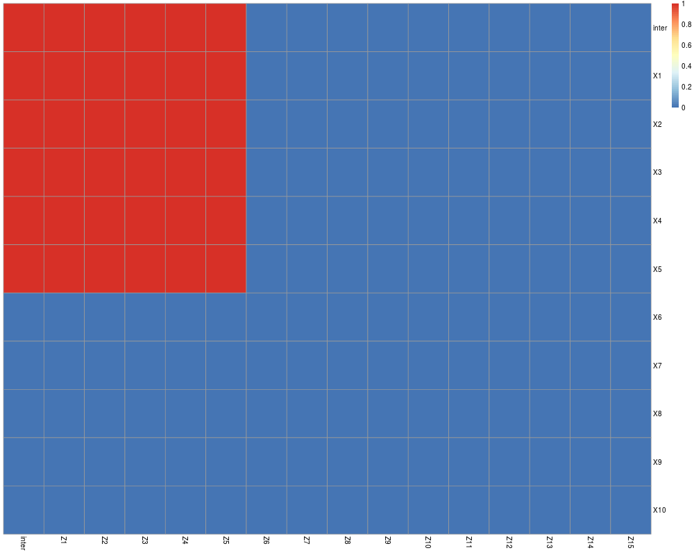
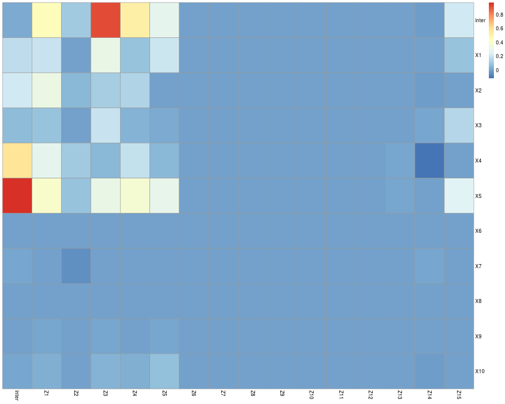
# First, we simulate data as follows:
# The first five features in X, and the first five features in Z, are non-zero.
# And given the non-zero main effects, all possible interactions are involved.
# We call this "high strong heredity"
B_high_SH<- B
B_high_SH[1:6,1:6]<- 1
#View true coefficient matrix
pheatmap(as.matrix(B_high_SH), scale="none",
cluster_rows=FALSE, cluster_cols=FALSE)
Y_high_SH <- as.vector(w.tr%*%as.vector(B_high_SH))+rnorm(100,sd = 2)
Y_high_SH.te <- as.vector(w.te%*%as.vector(B_high_SH))+rnorm(100,sd = 2)
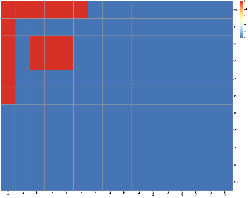
# Now a new setting:
# Again, the first five features in X, and the first five features in Z, are involved.
# But this time, only a subset of the possible interactions are involved.
# Strong heredity is still maintained.
# We call this "low strong heredity"
B_low_SH<- B_high_SH
B_low_SH[2:6,2:6]<-0
B_low_SH[3:4,3:5]<- 1
#View true coefficient matrix
pheatmap(as.matrix(B_low_SH), scale="none",
cluster_rows=FALSE, cluster_cols=FALSE)
Y_low_SH <- as.vector(w.tr%*%as.vector(B_low_SH))+rnorm(100,sd = 1.5)
Y_low_SH.te <- as.vector(w.te%*%as.vector(B_low_SH))+rnorm(100,sd = 1.5)
############################## FIT SOME MODELS ########################################
#Define alphas and lambdas
#Define 3 different alpha values
#Low alpha values penalize groups more
#High alpha values penalize individual Interactions more
alphas<- c(0.01,0.5,0.99)
lambdas<- seq(0.1,1,length = 50)
#high Strong heredity with l2 norm
fit_high_SH<- FAMILY(X.tr, Z.tr, Y_high_SH, lambdas ,
alphas, quad = TRUE,iter=500, verbose = TRUE )
yhat_hSH<- predict(fit_high_SH, X.te, Z.te)
mse_hSH <-apply(yhat_hSH,c(2,3), "-" ,Y_high_SH.te)
mse_hSH<- apply(mse_hSH^2,c(2,3),sum)
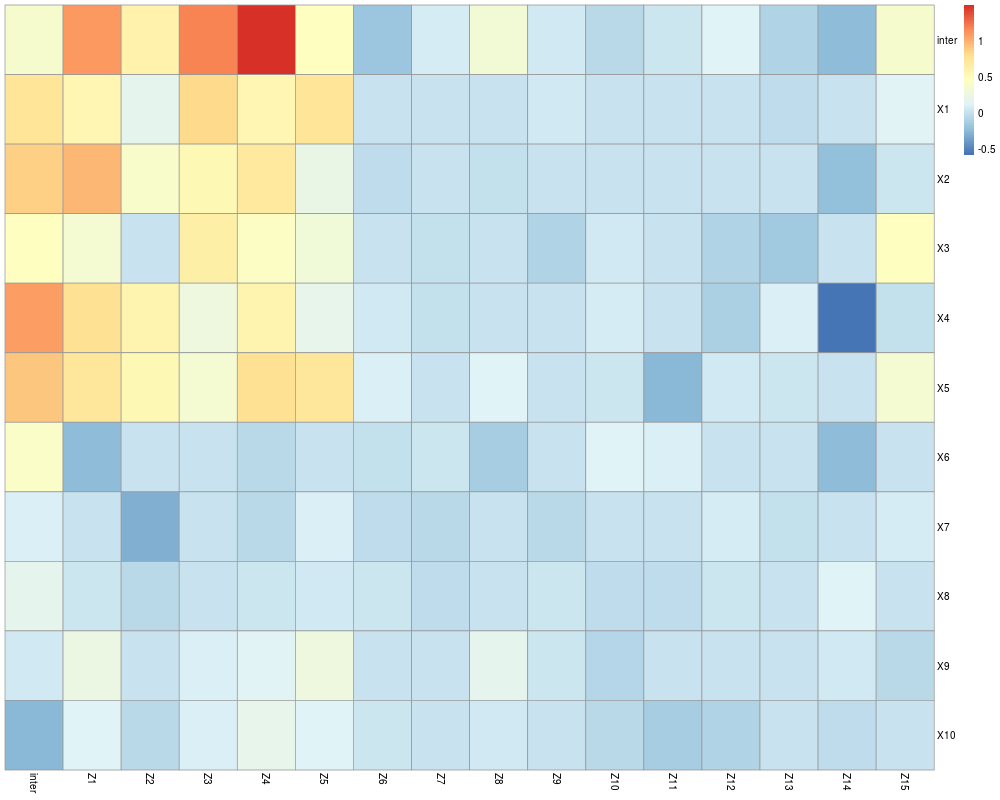
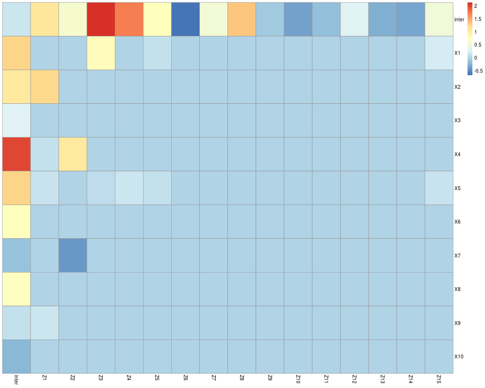
#Find optimal model and plot matrix
im<- which(mse_hSH==min(mse_hSH),TRUE)
plot(fit_high_SH$Estimate[[im[2] ]][[im[1]]])
#Plot some matrices for different alpha values
#Low alpha, higher penalty on groups
plot(fit_high_SH$Estimate[[ 1 ]][[ 25 ]])
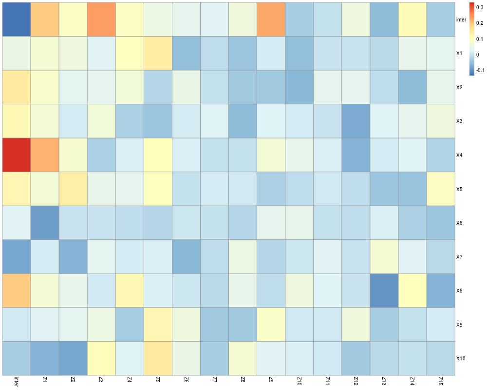
#Medium alpha, equal penalty on groups and individual interactions
plot(fit_high_SH$Estimate[[ 2 ]][[ 25 ]])
#High alpha, more penalty on individual interactions
plot(fit_high_SH$Estimate[[ 3 ]][[ 40 ]])
#View Coefficients
coef(fit_high_SH)[[im[2]]][[im[1]]]
############################## Uncomment code for EXAMPLE ###########################
# #high Strong heredity with l_infinity norm norm
# fit_high_SH<- FAMILY(X.tr, Z.tr, Y_high_SH, lambdas ,
# alphas, quad = TRUE,iter=500, verbose = TRUE,
# norm = "l_inf")
# yhat_hSH<- predict(fit_high_SH, X.te, Z.te)
# mse_hSH <-apply(yhat_hSH,c(2,3), "-" ,Y_high_SH.te)
# mse_hSH<- apply(mse_hSH^2,c(2,3),sum)
#
# #Find optimal model and plot matrix
# im<- which(mse_hSH==min(mse_hSH),TRUE)
# plot(fit_high_SH$Estimate[[im[2] ]][[im[1]]])
#
#
# #Plot some matrices for different alpha values
# #Low alpha, higher penalty on groups
# plot(fit_high_SH$Estimate[[ 1 ]][[ 30 ]])
# #Medium alpha, equal penalty on groups and individual interactions
# plot(fit_high_SH$Estimate[[ 2 ]][[ 10 ]])
# #High alpha, more penalty on individual interactions
# plot(fit_high_SH$Estimate[[ 3 ]][[ 20 ]])
#
#
# #View Coefficients
# coef(fit_high_SH)[[im[2]]][[im[1]]]
############################## Uncomment code for EXAMPLE ###########################
# #Redefine lambdas
# lambdas<- seq(0.1,0.5,length = 50)
#
# #low Strong heredity with l_2 norm
# fit_low_SH<- FAMILY(X.tr, Z.tr, Y_low_SH, lambdas ,
# alphas, quad = TRUE,iter=500, verbose = TRUE )
# yhat_lSH<- predict(fit_low_SH, X.te, Z.te)
# mse_lSH <-apply(yhat_lSH,c(2,3), "-" ,Y_low_SH.te)
# mse_lSH<- apply(mse_lSH^2,c(2,3),sum)
#
# #Find optimal model and plot matrix
# im<- which(mse_lSH==min(mse_lSH),TRUE)
# plot(fit_low_SH$Estimate[[im[2] ]][[im[1]]])
#
#
# #Plot some matrices for different alpha values
# #Low alpha, higher penalty on groups
# plot(fit_low_SH$Estimate[[ 1 ]][[ 25 ]])
# #Medium alpha, equal penalty on groups and individual interactions
# plot(fit_low_SH$Estimate[[ 2 ]][[ 10 ]])
# #High alpha, more penalty on individual interactions
# plot(fit_low_SH$Estimate[[ 3 ]][[ 10 ]])
#
#
# #View Coefficients
# coef(fit_low_SH)[[im[2]]][[im[1]]]
#####################################################################################
#####################################################################################
############################### EXAMPLE - BINARY RESPONSE ###########################
#####################################################################################
#####################################################################################
############################## GENERATE DATA ########################################
#Generate data for logistic regression
Yp_high_SH<- as.vector((w.tr)%*%as.vector(B_high_SH))
Yp_high_SH.te<- as.vector((w.te)%*%as.vector(B_high_SH))
Yprobs_high_SH<- 1/(1+exp(-Yp_high_SH))
Yprobs_high_SH.te<- 1/(1+exp(-Yp_high_SH.te))
Yp_high_SH<- rbinom(100, size = 1, prob = Yprobs_high_SH)
Yp_high_SH.te<- rbinom(100, size = 1, prob = Yprobs_high_SH.te)
lambdas<- seq(0.01,0.15,length = 50)
############################## FIT SOME MODELS ########################################
#Fit glm via l_2 norm
fit_high_SH<- FAMILY(X.tr, Z.tr, Yp_high_SH, lambdas ,
alphas, quad = TRUE,iter=500, verbose = TRUE,
family = "binomial")
yhp_hSH<- predict(fit_high_SH, X.te, Z.te)
mse_high_SH <-apply(yhp_hSH,c(2,3), "-" ,Yp_high_SH.te)
mse_hSH<- apply(mse_high_SH^2,c(2,3),sum)
im<- which(mse_hSH==min(mse_hSH),TRUE)
plot(fit_high_SH$Estimate[[im[2] ]][[im[1]]])
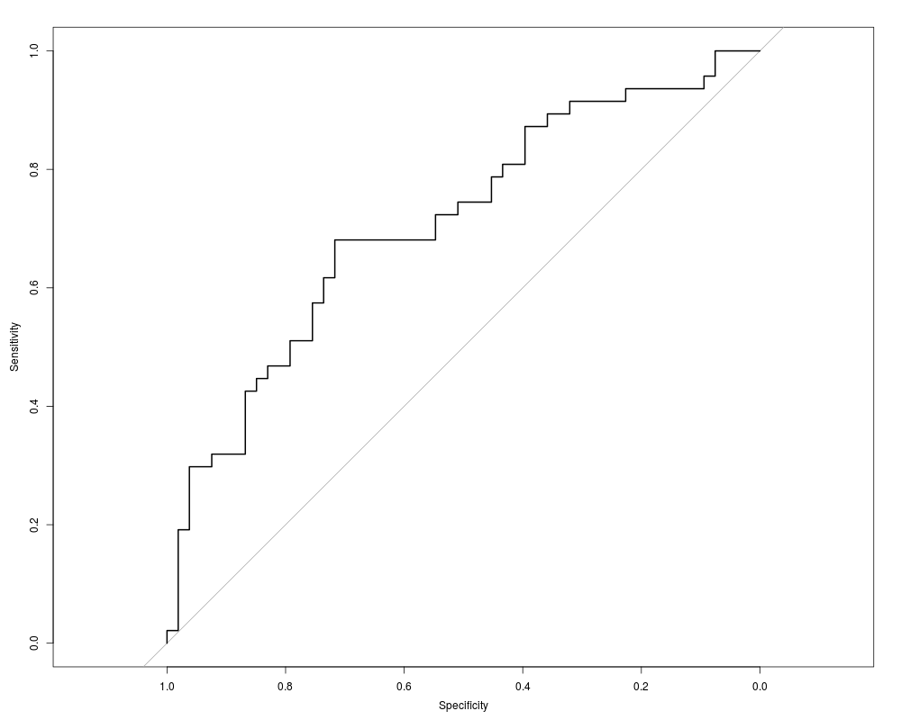
roc( Yp_high_SH.te,yhp_hSH[,im[1],im[2]],plot = TRUE)
#View Coefficients
coef(fit_high_SH)[[im[2]]][[im[1]]]
############################## Uncomment code for EXAMPLE ###########################
# #Fit glm via l_infinity norm
# fit_high_SH<- FAMILY(X.tr, Z.tr, Yp_high_SH, lambdas , norm = "l_inf",
# alphas, quad = TRUE,iter=500, verbose = TRUE,
# family = "binomial")
# yhp_hSH<- predict(fit_high_SH, X.te, Z.te)
# mse_high_SH <-apply(yhp_hSH,c(2,3), "-" ,Yp_high_SH.te)
# mse_hSH<- apply(mse_high_SH^2,c(2,3),sum)
# im<- which(mse_hSH==min(mse_hSH),TRUE)
# plot(fit_high_SH$Estimate[[im[2] ]][[im[1]]])
# roc( Yp_high_SH.te,yhp_hSH[,im[1],im[2]],plot = TRUE)
#
# #View Coefficients
# coef(fit_high_SH)[[im[2]]][[im[1]]]
#####################################################################################
#####################################################################################
############################## EXAMPLE WHERE X=Z ####################################
######################## Uncomment Code for EXAMPLE #################################
#####################################################################################
############################## GENERATE DATA ########################################
# #Redefine Lambdas
# lambdas<- seq(0.01,0.3,length = 50)
#
#
# #We consider the case X=Z now
# w.tr<- c()
# w.te<- c()
# X1<- cbind(1,X.tr)
# X2<- cbind(1,X.te)
#
# for(i in 1:11){
# for(j in 1:11){
# w.tr<- cbind(w.tr,X1[,j]*X1[,i])
# w.te<- cbind(w.te, X2[,j]*X2[,i])
# }
# }
#
# B<- matrix(0,ncol = 11,nrow = 11)
# rownames(B)<- c("inter" , paste("X",1:(nrow(B)-1),sep = ""))
# colnames(B)<- c("inter" , paste("X",1:(ncol(B)-1),sep = ""))
#
#
# B_high_SH<- B
# B_high_SH[1:6,1:6]<- 1
# #We exclude quadratic terms in this example
# diag(B_high_SH)[-1]<-0
# #View true coefficient matrix
# pheatmap(as.matrix(B_high_SH), scale="none",
# cluster_rows=FALSE, cluster_cols=FALSE)
#
# #With high Strong heredity: all possible interactions
# Y_high_SH <- as.vector(w.tr%*%as.vector(B_high_SH))+rnorm(100)
# Y_high_SH.te <- as.vector(w.te%*%as.vector(B_high_SH))+rnorm(100)
#
# ############################## FIT SOME MODELS ########################################
#
# #high Strong heredity with l_2 norm
# fit_high_SH<- FAMILY(X.tr, X.tr, Y_high_SH, lambdas ,
# alphas, quad = FALSE,iter=500, verbose = TRUE )
# yhat_hSH<- predict(fit_high_SH, X.te, X.te)
# mse_hSH <-apply(yhat_hSH,c(2,3), "-" ,Y_high_SH.te)
# mse_hSH<- apply(mse_hSH^2,c(2,3),sum)
#
# #Find optimal model and plot matrix
# im<- which(mse_hSH==min(mse_hSH),TRUE)
# plot(fit_high_SH$Estimate[[im[2] ]][[im[1]]])
#
#
# #Plot some matrices for different alpha values
# #Low alpha, higher penalty on groups
# plot(fit_high_SH$Estimate[[ 1 ]][[ 50 ]])
# #Medium alpha, equal penalty on groups and individual interactions
# plot(fit_high_SH$Estimate[[ 2 ]][[ 50 ]])
# #High alpha, more penalty on individual interactions
# plot(fit_high_SH$Estimate[[ 3 ]][[ 50 ]])
#
#
# #View Coefficients
# coef(fit_high_SH,XequalZ = TRUE)[[im[2]]][[im[1]]]
Results
R version 3.3.1 (2016-06-21) -- "Bug in Your Hair"
Copyright (C) 2016 The R Foundation for Statistical Computing
Platform: x86_64-pc-linux-gnu (64-bit)
R is free software and comes with ABSOLUTELY NO WARRANTY.
You are welcome to redistribute it under certain conditions.
Type 'license()' or 'licence()' for distribution details.
R is a collaborative project with many contributors.
Type 'contributors()' for more information and
'citation()' on how to cite R or R packages in publications.
Type 'demo()' for some demos, 'help()' for on-line help, or
'help.start()' for an HTML browser interface to help.
Type 'q()' to quit R.
> library(FAMILY)
> png(filename="/home/ddbj/snapshot/RGM3/R_CC/result/FAMILY/coef.FAMILY.Rd_%03d_medium.png", width=480, height=480)
> ### Name: coef.FAMILY
> ### Title: coef.FAMILY
> ### Aliases: coef.FAMILY
>
> ### ** Examples
>
> library(FAMILY)
> library(pROC)
Type 'citation("pROC")' for a citation.
Attaching package: 'pROC'
The following objects are masked from 'package:stats':
cov, smooth, var
> library(pheatmap)
>
> #####################################################################################
> #####################################################################################
> ############################# EXAMPLE - CONTINUOUS RESPONSE #########################
> #####################################################################################
> #####################################################################################
>
> ############################## GENERATE DATA ########################################
>
> #Generate training set of covariates X and Z
> set.seed(1)
> X.tr<- matrix(rnorm(10*100),ncol = 10, nrow = 100)
> Z.tr<- matrix(rnorm(15*100),ncol = 15, nrow = 100)
>
>
> #Generate test set of covariates X and Z
> X.te<- matrix(rnorm(10*100),ncol = 10, nrow = 100)
> Z.te<- matrix(rnorm(15*100),ncol = 15, nrow = 100)
>
> #Scale appropiately
> meanX<- apply(X.tr,2,mean)
> meanY<- apply(Z.tr,2,mean)
>
> X.tr<- scale(X.tr, scale = FALSE)
> Z.tr<- scale(Z.tr, scale = FALSE)
> X.te<- scale(X.te,center = meanX,scale = FALSE)
> Z.te<- scale(Z.te,center = meanY,scale = FALSE)
>
> #Generate full matrix of Covariates
> w.tr<- c()
> w.te<- c()
> X1<- cbind(1,X.tr)
> Z1<- cbind(1,Z.tr)
> X2<- cbind(1,X.te)
> Z2<- cbind(1,Z.te)
>
> for(i in 1:16){
+ for(j in 1:11){
+ w.tr<- cbind(w.tr,X1[,j]*Z1[,i])
+ w.te<- cbind(w.te, X2[,j]*Z2[,i])
+ }
+ }
>
> #Generate response variables with signal from
> #First 5 X features and 5 Z features.
>
> #We construct the coefficient matrix B.
> #B[1,1] contains the intercept
> #B[-1,1] contains the main effects for X.
> # For instance, B[2,1] is the main effect for the first feature in X.
> #B[1,-1] contains the main effects for Z.
> # For instance, B[1,10] is the coefficient for the 10th feature in Z.
> #B[i+1,j+1] is the coefficient of X_i Z_j
> B<- matrix(0,ncol = 16,nrow = 11)
> rownames(B)<- c("inter" , paste("X",1:(nrow(B)-1),sep = ""))
> colnames(B)<- c("inter" , paste("Z",1:(ncol(B)-1),sep = ""))
>
> # First, we simulate data as follows:
> # The first five features in X, and the first five features in Z, are non-zero.
> # And given the non-zero main effects, all possible interactions are involved.
> # We call this "high strong heredity"
> B_high_SH<- B
> B_high_SH[1:6,1:6]<- 1
> #View true coefficient matrix
> pheatmap(as.matrix(B_high_SH), scale="none",
+ cluster_rows=FALSE, cluster_cols=FALSE)
>
> Y_high_SH <- as.vector(w.tr%*%as.vector(B_high_SH))+rnorm(100,sd = 2)
> Y_high_SH.te <- as.vector(w.te%*%as.vector(B_high_SH))+rnorm(100,sd = 2)
>
> # Now a new setting:
> # Again, the first five features in X, and the first five features in Z, are involved.
> # But this time, only a subset of the possible interactions are involved.
> # Strong heredity is still maintained.
> # We call this "low strong heredity"
> B_low_SH<- B_high_SH
> B_low_SH[2:6,2:6]<-0
> B_low_SH[3:4,3:5]<- 1
> #View true coefficient matrix
> pheatmap(as.matrix(B_low_SH), scale="none",
+ cluster_rows=FALSE, cluster_cols=FALSE)
> Y_low_SH <- as.vector(w.tr%*%as.vector(B_low_SH))+rnorm(100,sd = 1.5)
> Y_low_SH.te <- as.vector(w.te%*%as.vector(B_low_SH))+rnorm(100,sd = 1.5)
>
>
> ############################## FIT SOME MODELS ########################################
>
> #Define alphas and lambdas
> #Define 3 different alpha values
> #Low alpha values penalize groups more
> #High alpha values penalize individual Interactions more
> alphas<- c(0.01,0.5,0.99)
> lambdas<- seq(0.1,1,length = 50)
>
> #high Strong heredity with l2 norm
> fit_high_SH<- FAMILY(X.tr, Z.tr, Y_high_SH, lambdas ,
+ alphas, quad = TRUE,iter=500, verbose = TRUE )
Computing w...done.
Starting svd...done.
Fitting model for alpha = 0.01 and lambda = 1
Fitting model for alpha = 0.01 and lambda = 0.98
Fitting model for alpha = 0.01 and lambda = 0.96
Fitting model for alpha = 0.01 and lambda = 0.94
Fitting model for alpha = 0.01 and lambda = 0.93
Fitting model for alpha = 0.01 and lambda = 0.91
Fitting model for alpha = 0.01 and lambda = 0.89
Fitting model for alpha = 0.01 and lambda = 0.87
Fitting model for alpha = 0.01 and lambda = 0.85
Fitting model for alpha = 0.01 and lambda = 0.83
Fitting model for alpha = 0.01 and lambda = 0.82
Fitting model for alpha = 0.01 and lambda = 0.8
Fitting model for alpha = 0.01 and lambda = 0.78
Fitting model for alpha = 0.01 and lambda = 0.76
Fitting model for alpha = 0.01 and lambda = 0.74
Fitting model for alpha = 0.01 and lambda = 0.72
Fitting model for alpha = 0.01 and lambda = 0.71
Fitting model for alpha = 0.01 and lambda = 0.69
Fitting model for alpha = 0.01 and lambda = 0.67
Fitting model for alpha = 0.01 and lambda = 0.65
Fitting model for alpha = 0.01 and lambda = 0.63
Fitting model for alpha = 0.01 and lambda = 0.61
Fitting model for alpha = 0.01 and lambda = 0.6
Fitting model for alpha = 0.01 and lambda = 0.58
Fitting model for alpha = 0.01 and lambda = 0.56
Fitting model for alpha = 0.01 and lambda = 0.54
Fitting model for alpha = 0.01 and lambda = 0.52
Fitting model for alpha = 0.01 and lambda = 0.5
Fitting model for alpha = 0.01 and lambda = 0.49
Fitting model for alpha = 0.01 and lambda = 0.47
Fitting model for alpha = 0.01 and lambda = 0.45
Fitting model for alpha = 0.01 and lambda = 0.43
Fitting model for alpha = 0.01 and lambda = 0.41
Fitting model for alpha = 0.01 and lambda = 0.39
Fitting model for alpha = 0.01 and lambda = 0.38
Fitting model for alpha = 0.01 and lambda = 0.36
Fitting model for alpha = 0.01 and lambda = 0.34
Fitting model for alpha = 0.01 and lambda = 0.32
Fitting model for alpha = 0.01 and lambda = 0.3
Fitting model for alpha = 0.01 and lambda = 0.28
Fitting model for alpha = 0.01 and lambda = 0.27
Fitting model for alpha = 0.01 and lambda = 0.25
Fitting model for alpha = 0.01 and lambda = 0.23
Fitting model for alpha = 0.01 and lambda = 0.21
Fitting model for alpha = 0.01 and lambda = 0.19
Fitting model for alpha = 0.01 and lambda = 0.17
Fitting model for alpha = 0.01 and lambda = 0.16
Fitting model for alpha = 0.01 and lambda = 0.14
Fitting model for alpha = 0.01 and lambda = 0.12
Fitting model for alpha = 0.01 and lambda = 0.1
Fitting model for alpha = 0.5 and lambda = 1
Fitting model for alpha = 0.5 and lambda = 0.98
Fitting model for alpha = 0.5 and lambda = 0.96
Fitting model for alpha = 0.5 and lambda = 0.94
Fitting model for alpha = 0.5 and lambda = 0.93
Fitting model for alpha = 0.5 and lambda = 0.91
Fitting model for alpha = 0.5 and lambda = 0.89
Fitting model for alpha = 0.5 and lambda = 0.87
Fitting model for alpha = 0.5 and lambda = 0.85
Fitting model for alpha = 0.5 and lambda = 0.83
Fitting model for alpha = 0.5 and lambda = 0.82
Fitting model for alpha = 0.5 and lambda = 0.8
Fitting model for alpha = 0.5 and lambda = 0.78
Fitting model for alpha = 0.5 and lambda = 0.76
Fitting model for alpha = 0.5 and lambda = 0.74
Fitting model for alpha = 0.5 and lambda = 0.72
Fitting model for alpha = 0.5 and lambda = 0.71
Fitting model for alpha = 0.5 and lambda = 0.69
Fitting model for alpha = 0.5 and lambda = 0.67
Fitting model for alpha = 0.5 and lambda = 0.65
Fitting model for alpha = 0.5 and lambda = 0.63
Fitting model for alpha = 0.5 and lambda = 0.61
Fitting model for alpha = 0.5 and lambda = 0.6
Fitting model for alpha = 0.5 and lambda = 0.58
Fitting model for alpha = 0.5 and lambda = 0.56
Fitting model for alpha = 0.5 and lambda = 0.54
Fitting model for alpha = 0.5 and lambda = 0.52
Fitting model for alpha = 0.5 and lambda = 0.5
Fitting model for alpha = 0.5 and lambda = 0.49
Fitting model for alpha = 0.5 and lambda = 0.47
Fitting model for alpha = 0.5 and lambda = 0.45
Fitting model for alpha = 0.5 and lambda = 0.43
Fitting model for alpha = 0.5 and lambda = 0.41
Fitting model for alpha = 0.5 and lambda = 0.39
Fitting model for alpha = 0.5 and lambda = 0.38
Fitting model for alpha = 0.5 and lambda = 0.36
Fitting model for alpha = 0.5 and lambda = 0.34
Fitting model for alpha = 0.5 and lambda = 0.32
Fitting model for alpha = 0.5 and lambda = 0.3
Fitting model for alpha = 0.5 and lambda = 0.28
Fitting model for alpha = 0.5 and lambda = 0.27
Fitting model for alpha = 0.5 and lambda = 0.25
Fitting model for alpha = 0.5 and lambda = 0.23
Fitting model for alpha = 0.5 and lambda = 0.21
Fitting model for alpha = 0.5 and lambda = 0.19
Fitting model for alpha = 0.5 and lambda = 0.17
Fitting model for alpha = 0.5 and lambda = 0.16
Fitting model for alpha = 0.5 and lambda = 0.14
Fitting model for alpha = 0.5 and lambda = 0.12
Fitting model for alpha = 0.5 and lambda = 0.1
Fitting model for alpha = 0.99 and lambda = 1
Fitting model for alpha = 0.99 and lambda = 0.98
Fitting model for alpha = 0.99 and lambda = 0.96
Fitting model for alpha = 0.99 and lambda = 0.94
Fitting model for alpha = 0.99 and lambda = 0.93
Fitting model for alpha = 0.99 and lambda = 0.91
Fitting model for alpha = 0.99 and lambda = 0.89
Fitting model for alpha = 0.99 and lambda = 0.87
Fitting model for alpha = 0.99 and lambda = 0.85
Fitting model for alpha = 0.99 and lambda = 0.83
Fitting model for alpha = 0.99 and lambda = 0.82
Fitting model for alpha = 0.99 and lambda = 0.8
Fitting model for alpha = 0.99 and lambda = 0.78
Fitting model for alpha = 0.99 and lambda = 0.76
Fitting model for alpha = 0.99 and lambda = 0.74
Fitting model for alpha = 0.99 and lambda = 0.72
Fitting model for alpha = 0.99 and lambda = 0.71
Fitting model for alpha = 0.99 and lambda = 0.69
Fitting model for alpha = 0.99 and lambda = 0.67
Fitting model for alpha = 0.99 and lambda = 0.65
Fitting model for alpha = 0.99 and lambda = 0.63
Fitting model for alpha = 0.99 and lambda = 0.61
Fitting model for alpha = 0.99 and lambda = 0.6
Fitting model for alpha = 0.99 and lambda = 0.58
Fitting model for alpha = 0.99 and lambda = 0.56
Fitting model for alpha = 0.99 and lambda = 0.54
Fitting model for alpha = 0.99 and lambda = 0.52
Fitting model for alpha = 0.99 and lambda = 0.5
Fitting model for alpha = 0.99 and lambda = 0.49
Fitting model for alpha = 0.99 and lambda = 0.47
Fitting model for alpha = 0.99 and lambda = 0.45
Fitting model for alpha = 0.99 and lambda = 0.43
Fitting model for alpha = 0.99 and lambda = 0.41
Fitting model for alpha = 0.99 and lambda = 0.39
Fitting model for alpha = 0.99 and lambda = 0.38
Fitting model for alpha = 0.99 and lambda = 0.36
Fitting model for alpha = 0.99 and lambda = 0.34
Fitting model for alpha = 0.99 and lambda = 0.32
Fitting model for alpha = 0.99 and lambda = 0.3
Fitting model for alpha = 0.99 and lambda = 0.28
Fitting model for alpha = 0.99 and lambda = 0.27
Fitting model for alpha = 0.99 and lambda = 0.25
Fitting model for alpha = 0.99 and lambda = 0.23
Fitting model for alpha = 0.99 and lambda = 0.21
Fitting model for alpha = 0.99 and lambda = 0.19
Fitting model for alpha = 0.99 and lambda = 0.17
Fitting model for alpha = 0.99 and lambda = 0.16
Fitting model for alpha = 0.99 and lambda = 0.14
Fitting model for alpha = 0.99 and lambda = 0.12
Fitting model for alpha = 0.99 and lambda = 0.1
> yhat_hSH<- predict(fit_high_SH, X.te, Z.te)
> mse_hSH <-apply(yhat_hSH,c(2,3), "-" ,Y_high_SH.te)
> mse_hSH<- apply(mse_hSH^2,c(2,3),sum)
>
> #Find optimal model and plot matrix
> im<- which(mse_hSH==min(mse_hSH),TRUE)
> plot(fit_high_SH$Estimate[[im[2] ]][[im[1]]])
>
>
> #Plot some matrices for different alpha values
> #Low alpha, higher penalty on groups
> plot(fit_high_SH$Estimate[[ 1 ]][[ 25 ]])
> #Medium alpha, equal penalty on groups and individual interactions
> plot(fit_high_SH$Estimate[[ 2 ]][[ 25 ]])
> #High alpha, more penalty on individual interactions
> plot(fit_high_SH$Estimate[[ 3 ]][[ 40 ]])
>
>
> #View Coefficients
> coef(fit_high_SH)[[im[2]]][[im[1]]]
$intercept
[1] 0.3660612
$mainsX
X Coef. est
[1,] 1 0.74106671
[2,] 2 0.87199302
[3,] 3 0.44399664
[4,] 4 1.06040396
[5,] 5 0.90672267
[6,] 6 0.39625494
[7,] 7 0.08497034
[8,] 8 0.17097666
[9,] 9 0.04380046
[10,] 10 -0.26754722
$mainsZ
Z Coef. est
[1,] 1 1.08763353
[2,] 2 0.58585423
[3,] 3 1.17322318
[4,] 4 1.49858095
[5,] 5 0.45218668
[6,] 6 -0.17905849
[7,] 7 0.07041749
[8,] 8 0.31521911
[9,] 9 0.04037807
[10,] 10 -0.06547316
[11,] 11 0.01708619
[12,] 12 0.11525280
[13,] 13 -0.10127333
[14,] 14 -0.25104818
[15,] 15 0.36484388
$interacts
X Z Coef. est
[1,] 1 1 0.5578295369
[2,] 1 2 0.1730776965
[3,] 1 3 0.8148027338
[4,] 1 4 0.5571329635
[5,] 1 5 0.7319715830
[6,] 1 9 0.0575240437
[7,] 1 13 -0.0347470090
[8,] 1 15 0.1352830738
[9,] 2 1 0.9619192679
[10,] 2 2 0.3812697455
[11,] 2 3 0.5303171103
[12,] 2 4 0.7044951294
[13,] 2 5 0.2083509789
[14,] 2 6 -0.0271647282
[15,] 2 8 -0.0163162853
[16,] 2 14 -0.2233279117
[17,] 2 15 0.0354304026
[18,] 3 1 0.3364459150
[19,] 3 3 0.6234262574
[20,] 3 4 0.4301907858
[21,] 3 5 0.2967603764
[22,] 3 7 -0.0063398846
[23,] 3 9 -0.1018623556
[24,] 3 10 0.0544570736
[25,] 3 12 -0.1035004436
[26,] 3 13 -0.1653631979
[27,] 3 15 0.4524197637
[28,] 4 1 0.7865778697
[29,] 4 2 0.5745010741
[30,] 4 3 0.2576428284
[31,] 4 4 0.5772894419
[32,] 4 5 0.1966229935
[33,] 4 6 0.0490099525
[34,] 4 7 -0.0135553939
[35,] 4 10 0.0767587686
[36,] 4 12 -0.1186453677
[37,] 4 13 0.0914928341
[38,] 4 14 -0.5885422895
[39,] 4 15 -0.0235524446
[40,] 5 1 0.7173233720
[41,] 5 2 0.5292900401
[42,] 5 3 0.3394433282
[43,] 5 4 0.7866571189
[44,] 5 5 0.7259235462
[45,] 5 6 0.0880023988
[46,] 5 8 0.1090425242
[47,] 5 9 0.0156231092
[48,] 5 10 0.0307094983
[49,] 5 11 -0.2548323690
[50,] 5 12 0.0523544449
[51,] 5 13 0.0353087829
[52,] 5 14 0.0024335982
[53,] 5 15 0.3332361674
[54,] 6 1 -0.2526241673
[55,] 6 4 -0.0629255692
[56,] 6 6 -0.0179481274
[57,] 6 7 0.0287249272
[58,] 6 8 -0.1330999551
[59,] 6 9 0.0077355010
[60,] 6 10 0.1117550753
[61,] 6 11 0.0947307799
[62,] 6 12 0.0028421409
[63,] 6 14 -0.2384378878
[64,] 6 15 -0.0007264793
[65,] 7 2 -0.3106003880
[66,] 7 4 -0.0554199954
[67,] 7 5 0.0896980472
[68,] 7 6 -0.0364820452
[69,] 7 7 -0.0471205773
[70,] 7 8 -0.0019636384
[71,] 7 9 -0.0548747534
[72,] 7 12 0.0661508313
[73,] 7 13 -0.0116683197
[74,] 7 15 0.0754463279
[75,] 8 1 0.0328937497
[76,] 8 2 -0.0606613635
[77,] 8 4 0.0177122799
[78,] 8 5 0.0427344484
[79,] 8 6 0.0229845376
[80,] 8 7 -0.0317311056
[81,] 8 9 0.0216367355
[82,] 8 10 -0.0377712252
[83,] 8 11 -0.0279991791
[84,] 8 12 0.0276992068
[85,] 8 13 0.0073108762
[86,] 8 14 0.1210525668
[87,] 9 1 0.2356221557
[88,] 9 2 0.0091461121
[89,] 9 3 0.0858649836
[90,] 9 4 0.1325265779
[91,] 9 5 0.2519507402
[92,] 9 6 0.0011115372
[93,] 9 8 0.1833241708
[94,] 9 9 0.0175746888
[95,] 9 10 -0.0824571059
[96,] 9 14 0.0474901846
[97,] 9 15 -0.0537351686
[98,] 10 1 0.1202347003
[99,] 10 2 -0.0636558169
[100,] 10 3 0.0976124448
[101,] 10 4 0.1847614426
[102,] 10 5 0.1111048832
[103,] 10 6 0.0219800374
[104,] 10 7 0.0125828537
[105,] 10 8 0.0551034109
[106,] 10 10 -0.0508601343
[107,] 10 11 -0.1371672610
[108,] 10 12 -0.1039230683
[109,] 10 14 -0.0416414647
$alpha
[1] 0.5
$lambda
[1] 0.1
>
> ############################## Uncomment code for EXAMPLE ###########################
> # #high Strong heredity with l_infinity norm norm
> # fit_high_SH<- FAMILY(X.tr, Z.tr, Y_high_SH, lambdas ,
> # alphas, quad = TRUE,iter=500, verbose = TRUE,
> # norm = "l_inf")
> # yhat_hSH<- predict(fit_high_SH, X.te, Z.te)
> # mse_hSH <-apply(yhat_hSH,c(2,3), "-" ,Y_high_SH.te)
> # mse_hSH<- apply(mse_hSH^2,c(2,3),sum)
> #
> # #Find optimal model and plot matrix
> # im<- which(mse_hSH==min(mse_hSH),TRUE)
> # plot(fit_high_SH$Estimate[[im[2] ]][[im[1]]])
> #
> #
> # #Plot some matrices for different alpha values
> # #Low alpha, higher penalty on groups
> # plot(fit_high_SH$Estimate[[ 1 ]][[ 30 ]])
> # #Medium alpha, equal penalty on groups and individual interactions
> # plot(fit_high_SH$Estimate[[ 2 ]][[ 10 ]])
> # #High alpha, more penalty on individual interactions
> # plot(fit_high_SH$Estimate[[ 3 ]][[ 20 ]])
> #
> #
> # #View Coefficients
> # coef(fit_high_SH)[[im[2]]][[im[1]]]
>
>
> ############################## Uncomment code for EXAMPLE ###########################
> # #Redefine lambdas
> # lambdas<- seq(0.1,0.5,length = 50)
> #
> # #low Strong heredity with l_2 norm
> # fit_low_SH<- FAMILY(X.tr, Z.tr, Y_low_SH, lambdas ,
> # alphas, quad = TRUE,iter=500, verbose = TRUE )
> # yhat_lSH<- predict(fit_low_SH, X.te, Z.te)
> # mse_lSH <-apply(yhat_lSH,c(2,3), "-" ,Y_low_SH.te)
> # mse_lSH<- apply(mse_lSH^2,c(2,3),sum)
> #
> # #Find optimal model and plot matrix
> # im<- which(mse_lSH==min(mse_lSH),TRUE)
> # plot(fit_low_SH$Estimate[[im[2] ]][[im[1]]])
> #
> #
> # #Plot some matrices for different alpha values
> # #Low alpha, higher penalty on groups
> # plot(fit_low_SH$Estimate[[ 1 ]][[ 25 ]])
> # #Medium alpha, equal penalty on groups and individual interactions
> # plot(fit_low_SH$Estimate[[ 2 ]][[ 10 ]])
> # #High alpha, more penalty on individual interactions
> # plot(fit_low_SH$Estimate[[ 3 ]][[ 10 ]])
> #
> #
> # #View Coefficients
> # coef(fit_low_SH)[[im[2]]][[im[1]]]
>
>
> #####################################################################################
> #####################################################################################
> ############################### EXAMPLE - BINARY RESPONSE ###########################
> #####################################################################################
> #####################################################################################
>
> ############################## GENERATE DATA ########################################
>
> #Generate data for logistic regression
> Yp_high_SH<- as.vector((w.tr)%*%as.vector(B_high_SH))
> Yp_high_SH.te<- as.vector((w.te)%*%as.vector(B_high_SH))
>
> Yprobs_high_SH<- 1/(1+exp(-Yp_high_SH))
> Yprobs_high_SH.te<- 1/(1+exp(-Yp_high_SH.te))
>
> Yp_high_SH<- rbinom(100, size = 1, prob = Yprobs_high_SH)
> Yp_high_SH.te<- rbinom(100, size = 1, prob = Yprobs_high_SH.te)
>
> lambdas<- seq(0.01,0.15,length = 50)
>
> ############################## FIT SOME MODELS ########################################
>
> #Fit glm via l_2 norm
> fit_high_SH<- FAMILY(X.tr, Z.tr, Yp_high_SH, lambdas ,
+ alphas, quad = TRUE,iter=500, verbose = TRUE,
+ family = "binomial")
Computing w...done.
Starting svd...done.
Fitting model for alpha = 0.01 and lambda = 0.15
Fitting model for alpha = 0.01 and lambda = 0.15
Fitting model for alpha = 0.01 and lambda = 0.14
Fitting model for alpha = 0.01 and lambda = 0.14
Fitting model for alpha = 0.01 and lambda = 0.14
Fitting model for alpha = 0.01 and lambda = 0.14
Fitting model for alpha = 0.01 and lambda = 0.13
Fitting model for alpha = 0.01 and lambda = 0.13
Fitting model for alpha = 0.01 and lambda = 0.13
Fitting model for alpha = 0.01 and lambda = 0.12
Fitting model for alpha = 0.01 and lambda = 0.12
Fitting model for alpha = 0.01 and lambda = 0.12
Fitting model for alpha = 0.01 and lambda = 0.12
Fitting model for alpha = 0.01 and lambda = 0.11
Fitting model for alpha = 0.01 and lambda = 0.11
Fitting model for alpha = 0.01 and lambda = 0.11
Fitting model for alpha = 0.01 and lambda = 0.1
Fitting model for alpha = 0.01 and lambda = 0.1
Fitting model for alpha = 0.01 and lambda = 0.1
Fitting model for alpha = 0.01 and lambda = 0.1
Fitting model for alpha = 0.01 and lambda = 0.09
Fitting model for alpha = 0.01 and lambda = 0.09
Fitting model for alpha = 0.01 and lambda = 0.09
Fitting model for alpha = 0.01 and lambda = 0.08
Fitting model for alpha = 0.01 and lambda = 0.08
Fitting model for alpha = 0.01 and lambda = 0.08
Fitting model for alpha = 0.01 and lambda = 0.08
Fitting model for alpha = 0.01 and lambda = 0.07
Fitting model for alpha = 0.01 and lambda = 0.07
Fitting model for alpha = 0.01 and lambda = 0.07
Fitting model for alpha = 0.01 and lambda = 0.06
Fitting model for alpha = 0.01 and lambda = 0.06
Fitting model for alpha = 0.01 and lambda = 0.06
Fitting model for alpha = 0.01 and lambda = 0.06
Fitting model for alpha = 0.01 and lambda = 0.05
Fitting model for alpha = 0.01 and lambda = 0.05
Fitting model for alpha = 0.01 and lambda = 0.05
Fitting model for alpha = 0.01 and lambda = 0.04
Fitting model for alpha = 0.01 and lambda = 0.04
Fitting model for alpha = 0.01 and lambda = 0.04
Fitting model for alpha = 0.01 and lambda = 0.04
Fitting model for alpha = 0.01 and lambda = 0.03
Fitting model for alpha = 0.01 and lambda = 0.03
Fitting model for alpha = 0.01 and lambda = 0.03
Fitting model for alpha = 0.01 and lambda = 0.02
Fitting model for alpha = 0.01 and lambda = 0.02
Fitting model for alpha = 0.01 and lambda = 0.02
Fitting model for alpha = 0.01 and lambda = 0.02
Fitting model for alpha = 0.01 and lambda = 0.01
Fitting model for alpha = 0.01 and lambda = 0.01
Fitting model for alpha = 0.5 and lambda = 0.15
Fitting model for alpha = 0.5 and lambda = 0.15
Fitting model for alpha = 0.5 and lambda = 0.14
Fitting model for alpha = 0.5 and lambda = 0.14
Fitting model for alpha = 0.5 and lambda = 0.14
Fitting model for alpha = 0.5 and lambda = 0.14
Fitting model for alpha = 0.5 and lambda = 0.13
Fitting model for alpha = 0.5 and lambda = 0.13
Fitting model for alpha = 0.5 and lambda = 0.13
Fitting model for alpha = 0.5 and lambda = 0.12
Fitting model for alpha = 0.5 and lambda = 0.12
Fitting model for alpha = 0.5 and lambda = 0.12
Fitting model for alpha = 0.5 and lambda = 0.12
Fitting model for alpha = 0.5 and lambda = 0.11
Fitting model for alpha = 0.5 and lambda = 0.11
Fitting model for alpha = 0.5 and lambda = 0.11
Fitting model for alpha = 0.5 and lambda = 0.1
Fitting model for alpha = 0.5 and lambda = 0.1
Fitting model for alpha = 0.5 and lambda = 0.1
Fitting model for alpha = 0.5 and lambda = 0.1
Fitting model for alpha = 0.5 and lambda = 0.09
Fitting model for alpha = 0.5 and lambda = 0.09
Fitting model for alpha = 0.5 and lambda = 0.09
Fitting model for alpha = 0.5 and lambda = 0.08
Fitting model for alpha = 0.5 and lambda = 0.08
Fitting model for alpha = 0.5 and lambda = 0.08
Fitting model for alpha = 0.5 and lambda = 0.08
Fitting model for alpha = 0.5 and lambda = 0.07
Fitting model for alpha = 0.5 and lambda = 0.07
Fitting model for alpha = 0.5 and lambda = 0.07
Fitting model for alpha = 0.5 and lambda = 0.06
Fitting model for alpha = 0.5 and lambda = 0.06
Fitting model for alpha = 0.5 and lambda = 0.06
Fitting model for alpha = 0.5 and lambda = 0.06
Fitting model for alpha = 0.5 and lambda = 0.05
Fitting model for alpha = 0.5 and lambda = 0.05
Fitting model for alpha = 0.5 and lambda = 0.05
Fitting model for alpha = 0.5 and lambda = 0.04
Fitting model for alpha = 0.5 and lambda = 0.04
Fitting model for alpha = 0.5 and lambda = 0.04
Fitting model for alpha = 0.5 and lambda = 0.04
Fitting model for alpha = 0.5 and lambda = 0.03
Fitting model for alpha = 0.5 and lambda = 0.03
Fitting model for alpha = 0.5 and lambda = 0.03
Fitting model for alpha = 0.5 and lambda = 0.02
Fitting model for alpha = 0.5 and lambda = 0.02
Fitting model for alpha = 0.5 and lambda = 0.02
Fitting model for alpha = 0.5 and lambda = 0.02
Fitting model for alpha = 0.5 and lambda = 0.01
Fitting model for alpha = 0.5 and lambda = 0.01
Fitting model for alpha = 0.99 and lambda = 0.15
Fitting model for alpha = 0.99 and lambda = 0.15
Fitting model for alpha = 0.99 and lambda = 0.14
Fitting model for alpha = 0.99 and lambda = 0.14
Fitting model for alpha = 0.99 and lambda = 0.14
Fitting model for alpha = 0.99 and lambda = 0.14
Fitting model for alpha = 0.99 and lambda = 0.13
Fitting model for alpha = 0.99 and lambda = 0.13
Fitting model for alpha = 0.99 and lambda = 0.13
Fitting model for alpha = 0.99 and lambda = 0.12
Fitting model for alpha = 0.99 and lambda = 0.12
Fitting model for alpha = 0.99 and lambda = 0.12
Fitting model for alpha = 0.99 and lambda = 0.12
Fitting model for alpha = 0.99 and lambda = 0.11
Fitting model for alpha = 0.99 and lambda = 0.11
Fitting model for alpha = 0.99 and lambda = 0.11
Fitting model for alpha = 0.99 and lambda = 0.1
Fitting model for alpha = 0.99 and lambda = 0.1
Fitting model for alpha = 0.99 and lambda = 0.1
Fitting model for alpha = 0.99 and lambda = 0.1
Fitting model for alpha = 0.99 and lambda = 0.09
Fitting model for alpha = 0.99 and lambda = 0.09
Fitting model for alpha = 0.99 and lambda = 0.09
Fitting model for alpha = 0.99 and lambda = 0.08
Fitting model for alpha = 0.99 and lambda = 0.08
Fitting model for alpha = 0.99 and lambda = 0.08
Fitting model for alpha = 0.99 and lambda = 0.08
Fitting model for alpha = 0.99 and lambda = 0.07
Fitting model for alpha = 0.99 and lambda = 0.07
Fitting model for alpha = 0.99 and lambda = 0.07
Fitting model for alpha = 0.99 and lambda = 0.06
Fitting model for alpha = 0.99 and lambda = 0.06
Fitting model for alpha = 0.99 and lambda = 0.06
Fitting model for alpha = 0.99 and lambda = 0.06
Fitting model for alpha = 0.99 and lambda = 0.05
Fitting model for alpha = 0.99 and lambda = 0.05
Fitting model for alpha = 0.99 and lambda = 0.05
Fitting model for alpha = 0.99 and lambda = 0.04
Fitting model for alpha = 0.99 and lambda = 0.04
Fitting model for alpha = 0.99 and lambda = 0.04
Fitting model for alpha = 0.99 and lambda = 0.04
Fitting model for alpha = 0.99 and lambda = 0.03
Fitting model for alpha = 0.99 and lambda = 0.03
Fitting model for alpha = 0.99 and lambda = 0.03
Fitting model for alpha = 0.99 and lambda = 0.02
Fitting model for alpha = 0.99 and lambda = 0.02
Fitting model for alpha = 0.99 and lambda = 0.02
Fitting model for alpha = 0.99 and lambda = 0.02
Fitting model for alpha = 0.99 and lambda = 0.01
Fitting model for alpha = 0.99 and lambda = 0.01
> yhp_hSH<- predict(fit_high_SH, X.te, Z.te)
> mse_high_SH <-apply(yhp_hSH,c(2,3), "-" ,Yp_high_SH.te)
> mse_hSH<- apply(mse_high_SH^2,c(2,3),sum)
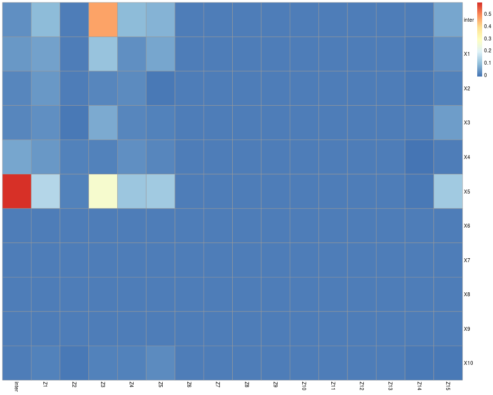
> im<- which(mse_hSH==min(mse_hSH),TRUE)
> plot(fit_high_SH$Estimate[[im[2] ]][[im[1]]])
> roc( Yp_high_SH.te,yhp_hSH[,im[1],im[2]],plot = TRUE)
Call:
roc.default(response = Yp_high_SH.te, predictor = yhp_hSH[, im[1], im[2]], plot = TRUE)
Data: yhp_hSH[, im[1], im[2]] in 53 controls (Yp_high_SH.te 0) < 47 cases (Yp_high_SH.te 1).
Area under the curve: 0.7098
>
> #View Coefficients
> coef(fit_high_SH)[[im[2]]][[im[1]]]
$intercept
[1] -0.1343509
$mainsX
X Coef. est
[1,] 1 0.045038330
[2,] 2 0.148037466
[3,] 3 0.114267346
[4,] 4 0.332174924
[5,] 5 0.118598318
[6,] 6 0.025698165
[7,] 7 -0.078534321
[8,] 8 0.195587464
[9,] 9 0.005813525
[10,] 10 -0.035811651
$mainsZ
Z Coef. est
[1,] 1 0.195389413
[2,] 2 0.092241016
[3,] 3 0.236739448
[4,] 4 0.093706527
[5,] 5 0.050980386
[6,] 6 0.036939084
[7,] 7 0.024893747
[8,] 8 0.061117695
[9,] 9 0.228266733
[10,] 10 -0.035257505
[11,] 11 -0.005023177
[12,] 12 0.056650246
[13,] 13 -0.055493851
[14,] 14 0.108600101
[15,] 15 -0.032966232
$interacts
X Z Coef. est
[1,] 1 1 7.482233e-02
[2,] 1 2 5.330181e-02
[3,] 1 3 2.850806e-02
[4,] 1 4 9.449871e-02
[5,] 1 5 1.427534e-01
[6,] 1 6 -5.140860e-02
[7,] 1 7 -1.113753e-02
[8,] 1 8 -4.477706e-02
[9,] 1 9 1.118885e-02
[10,] 1 10 -5.227674e-02
[11,] 1 11 -2.428516e-03
[12,] 1 12 1.869408e-05
[13,] 1 13 -1.411863e-02
[14,] 1 14 4.198845e-02
[15,] 1 15 2.967011e-02
[16,] 2 1 8.409200e-02
[17,] 2 2 3.162097e-02
[18,] 2 3 3.670323e-02
[19,] 2 4 6.416572e-02
[20,] 2 5 -2.084966e-02
[21,] 2 6 4.667051e-02
[22,] 2 7 -5.591183e-03
[23,] 2 8 -4.070916e-02
[24,] 2 9 -3.957131e-02
[25,] 2 10 -6.020412e-02
[26,] 2 11 3.722022e-02
[27,] 2 12 3.797098e-02
[28,] 2 13 -1.133050e-02
[29,] 2 14 -5.697230e-02
[30,] 2 15 4.022022e-02
[31,] 3 1 6.968112e-02
[32,] 3 2 1.269424e-02
[33,] 3 3 6.585108e-02
[34,] 3 4 -2.790849e-02
[35,] 3 5 -4.439406e-02
[36,] 3 6 1.063517e-02
[37,] 3 7 2.236860e-02
[38,] 3 8 -5.929593e-02
[39,] 3 9 2.216973e-02
[40,] 3 10 1.330013e-02
[41,] 3 11 8.563777e-05
[42,] 3 12 -7.720376e-02
[43,] 3 13 2.124283e-02
[44,] 3 14 3.820089e-02
[45,] 3 15 5.401901e-02
[46,] 4 1 2.162890e-01
[47,] 4 2 7.562473e-02
[48,] 4 3 -2.781269e-02
[49,] 4 4 1.612130e-02
[50,] 4 5 1.014177e-01
[51,] 4 6 1.659543e-02
[52,] 4 7 -4.711454e-03
|