Supported by Dr. Osamu Ogasawara and  . . |
|
Last data update: 2014.03.03 |
Fast Kalman filterDescriptionThis function allows for fast and flexible Kalman filtering. Both, the
measurement and transition equation may be multivariate and parameters
are allowed to be time-varying. In addition “NA”-values in the
observations are supported. Usagefkf(a0, P0, dt, ct, Tt, Zt, HHt, GGt, yt, check.input = TRUE) Arguments
DetailsState space form: The following notation is closest to the one of Koopman et al. The state space model is represented by the transition equation and the measurement equation. Let m be the dimension of the state variable, d be the dimension of the observations, and n the number of observations. The transition equation and the measurement equation are given by alpha(t + 1) = d(t) + T(t) alpha(t) + H(t) * eta(t) y(t) = c(t) + Z(t) alpha(t) + G(t) * epsilon(t), where eta(t) and epsilon(t) are iid N(0, I(m)) and iid N(0, I(d)), respectively, and alpha(t) denotes the state variable. The parameters admit the following dimensions:
Note that Iteration: Let Initialization: Updating equations: Prediction equations: Next iteration: NA-values: NA-values in the observation matrix Parameters: The parameters can either be constant or deterministic time-varying. Assume the number of observations is n (i.e. y = y[,1:n]). Then, the parameters admit the following classes and dimensions:
If BLAS and LAPACK routines used: The R function
The only critical part is to compute the inverse of F[,,t]
and the determinant of F[,,t]. If the inverse can not be
computed, the filter stops and returns the corresponding message in
The inverse is computed in
two steps: First, the Cholesky factorization of F[,,t] is
calculated by ValueAn S3-object of class “fkf”, which is a list with the following elements:
The first element of both Author(s)David Luethi Philipp Erb Simon Otziger Maintainer: Philipp Erb <erb.philipp@gmail.com> ReferencesHarvey, Andrew C. (1990). Forecasting, Structural Time Series Models and the Kalman Filter. Cambridge University Press. Hamilton, James D. (1994). Time Series Analysis. Princeton University Press. Koopman, S. J., Shephard, N., Doornik, J. A. (1999). Statistical algorithms for models in state space using SsfPack 2.2. Econometrics Journal, Royal Economic Society, vol. 2(1), pages 107-160. See Also
Examples
## <--------------------------------------------------------------------------->
## Example 1: ARMA(2, 1) model estimation.
## <--------------------------------------------------------------------------->
## This example shows how to fit an ARMA(2, 1) model using this Kalman
## filter implementation (see also stats' makeARIMA and KalmanRun).
n <- 1000
## Set the AR parameters
ar1 <- 0.6
ar2 <- 0.2
ma1 <- -0.2
sigma <- sqrt(0.2)
## Sample from an ARMA(2, 1) process
a <- arima.sim(model = list(ar = c(ar1, ar2), ma = ma1), n = n,
innov = rnorm(n) * sigma)
## Create a state space representation out of the four ARMA parameters
arma21ss <- function(ar1, ar2, ma1, sigma) {
Tt <- matrix(c(ar1, ar2, 1, 0), ncol = 2)
Zt <- matrix(c(1, 0), ncol = 2)
ct <- matrix(0)
dt <- matrix(0, nrow = 2)
GGt <- matrix(0)
H <- matrix(c(1, ma1), nrow = 2) * sigma
HHt <- H %*% t(H)
a0 <- c(0, 0)
P0 <- matrix(1e6, nrow = 2, ncol = 2)
return(list(a0 = a0, P0 = P0, ct = ct, dt = dt, Zt = Zt, Tt = Tt, GGt = GGt,
HHt = HHt))
}
## The objective function passed to 'optim'
objective <- function(theta, yt) {
sp <- arma21ss(theta["ar1"], theta["ar2"], theta["ma1"], theta["sigma"])
ans <- fkf(a0 = sp$a0, P0 = sp$P0, dt = sp$dt, ct = sp$ct, Tt = sp$Tt,
Zt = sp$Zt, HHt = sp$HHt, GGt = sp$GGt, yt = yt)
return(-ans$logLik)
}
theta <- c(ar = c(0, 0), ma1 = 0, sigma = 1)
fit <- optim(theta, objective, yt = rbind(a), hessian = TRUE)
fit
## Confidence intervals
rbind(fit$par - qnorm(0.975) * sqrt(diag(solve(fit$hessian))),
fit$par + qnorm(0.975) * sqrt(diag(solve(fit$hessian))))
## Filter the series with estimated parameter values
sp <- arma21ss(fit$par["ar1"], fit$par["ar2"], fit$par["ma1"], fit$par["sigma"])
ans <- fkf(a0 = sp$a0, P0 = sp$P0, dt = sp$dt, ct = sp$ct, Tt = sp$Tt,
Zt = sp$Zt, HHt = sp$HHt, GGt = sp$GGt, yt = rbind(a))
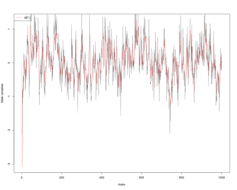
## Compare the prediction with the realization
plot(ans, at.idx = 1, att.idx = NA, CI = NA)
lines(a, lty = "dotted")
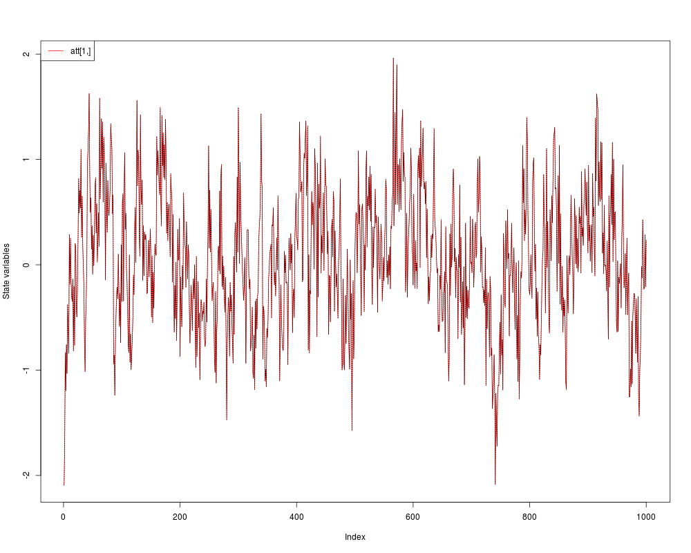
## Compare the filtered series with the realization
plot(ans, at.idx = NA, att.idx = 1, CI = NA)
lines(a, lty = "dotted")
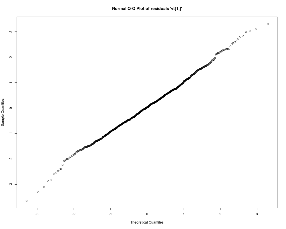
## Check whether the residuals are Gaussian
plot(ans, type = "resid.qq")
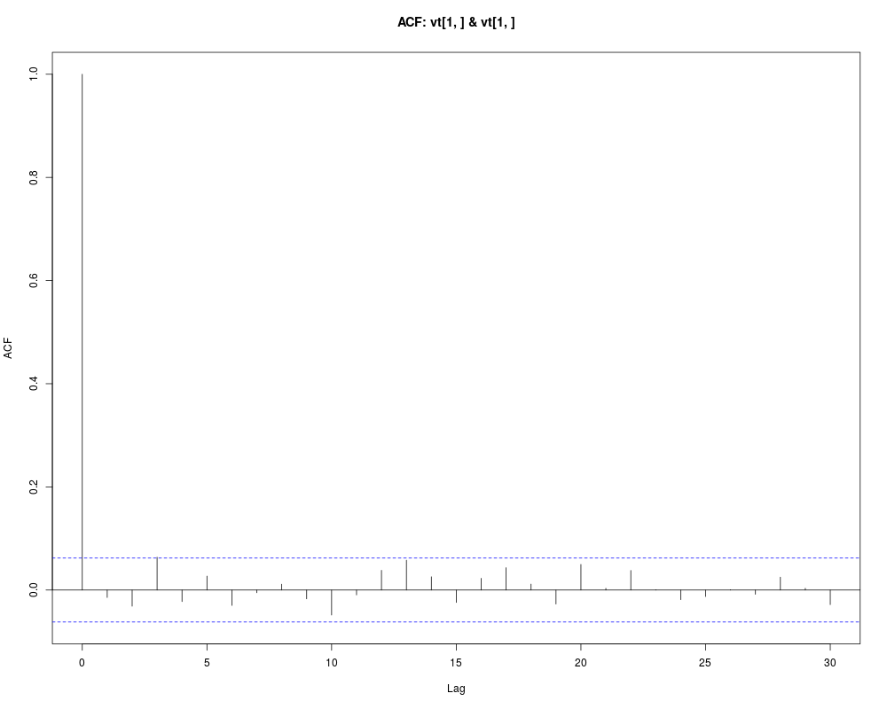
## Check for linear serial dependence through 'acf'
plot(ans, type = "acf")
## <--------------------------------------------------------------------------->
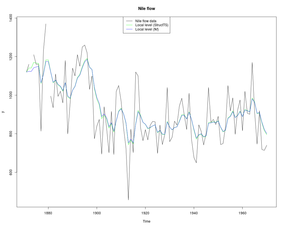
## Example 2: Local level model for the Nile's annual flow.
## <--------------------------------------------------------------------------->
## Transition equation:
## alpha[t+1] = alpha[t] + eta[t], eta[t] ~ N(0, HHt)
## Measurement equation:
## y[t] = alpha[t] + eps[t], eps[t] ~ N(0, GGt)
y <- Nile
y[c(3, 10)] <- NA # NA values can be handled
## Set constant parameters:
dt <- ct <- matrix(0)
Zt <- Tt <- matrix(1)
a0 <- y[1] # Estimation of the first year flow
P0 <- matrix(100) # Variance of 'a0'
## Estimate parameters:
fit.fkf <- optim(c(HHt = var(y, na.rm = TRUE) * .5,
GGt = var(y, na.rm = TRUE) * .5),
fn = function(par, ...)
-fkf(HHt = matrix(par[1]), GGt = matrix(par[2]), ...)$logLik,
yt = rbind(y), a0 = a0, P0 = P0, dt = dt, ct = ct,
Zt = Zt, Tt = Tt, check.input = FALSE)
## Filter Nile data with estimated parameters:
fkf.obj <- fkf(a0, P0, dt, ct, Tt, Zt, HHt = matrix(fit.fkf$par[1]),
GGt = matrix(fit.fkf$par[2]), yt = rbind(y))
## Compare with the stats' structural time series implementation:
fit.stats <- StructTS(y, type = "level")
fit.fkf$par
fit.stats$coef
## Plot the flow data together with fitted local levels:
plot(y, main = "Nile flow")
lines(fitted(fit.stats), col = "green")
lines(ts(fkf.obj$att[1, ], start = start(y), frequency = frequency(y)), col = "blue")
legend("top", c("Nile flow data", "Local level (StructTS)", "Local level (fkf)"),
col = c("black", "green", "blue"), lty = 1)
Results
R version 3.3.1 (2016-06-21) -- "Bug in Your Hair"
Copyright (C) 2016 The R Foundation for Statistical Computing
Platform: x86_64-pc-linux-gnu (64-bit)

R is free software and comes with ABSOLUTELY NO WARRANTY.
You are welcome to redistribute it under certain conditions.
Type 'license()' or 'licence()' for distribution details.

R is a collaborative project with many contributors.
Type 'contributors()' for more information and
'citation()' on how to cite R or R packages in publications.

Type 'demo()' for some demos, 'help()' for on-line help, or
'help.start()' for an HTML browser interface to help.
Type 'q()' to quit R.

> library(FKF)
Loading required package: RUnit
> png(filename="/home/ddbj/snapshot/RGM3/R_CC/result/FKF/fkf.Rd_%03d_medium.png", width=480, height=480)
> ### Name: fkf
> ### Title: Fast Kalman filter
> ### Aliases: fkf
> ### Keywords: algebra models multivariate
>
> ### ** Examples
>
> ## <--------------------------------------------------------------------------->
> ## Example 1: ARMA(2, 1) model estimation.
> ## <--------------------------------------------------------------------------->
> ## This example shows how to fit an ARMA(2, 1) model using this Kalman
> ## filter implementation (see also stats' makeARIMA and KalmanRun).
> n <- 1000
>
> ## Set the AR parameters
> ar1 <- 0.6
> ar2 <- 0.2
> ma1 <- -0.2
> sigma <- sqrt(0.2)
>
> ## Sample from an ARMA(2, 1) process
> a <- arima.sim(model = list(ar = c(ar1, ar2), ma = ma1), n = n,
+                innov = rnorm(n) * sigma)
>
> ## Create a state space representation out of the four ARMA parameters
> arma21ss <- function(ar1, ar2, ma1, sigma) {
+     Tt <- matrix(c(ar1, ar2, 1, 0), ncol = 2)
+     Zt <- matrix(c(1, 0), ncol = 2)
+     ct <- matrix(0)
+     dt <- matrix(0, nrow = 2)
+     GGt <- matrix(0)
+     H <- matrix(c(1, ma1), nrow = 2) * sigma
+     HHt <- H %*% t(H)
+     a0 <- c(0, 0)
+     P0 <- matrix(1e6, nrow = 2, ncol = 2)
+     return(list(a0 = a0, P0 = P0, ct = ct, dt = dt, Zt = Zt, Tt = Tt, GGt = GGt,
+                 HHt = HHt))
+ }
>
> ## The objective function passed to 'optim'
> objective <- function(theta, yt) {
+     sp <- arma21ss(theta["ar1"], theta["ar2"], theta["ma1"], theta["sigma"])
+     ans <- fkf(a0 = sp$a0, P0 = sp$P0, dt = sp$dt, ct = sp$ct, Tt = sp$Tt,
+                Zt = sp$Zt, HHt = sp$HHt, GGt = sp$GGt, yt = yt)
+     return(-ans$logLik)
+ }
>
> theta <- c(ar = c(0, 0), ma1 = 0, sigma = 1)
> fit <- optim(theta, objective, yt = rbind(a), hessian = TRUE)
> fit
$par
       ar1        ar2        ma1      sigma
 0.5039113  0.2597601 -0.1039661  0.4415869

$value
[1] 608.7166

$counts
function gradient
     331       NA

$convergence
[1] 0

$message
NULL

$hessian
                ar1          ar2          ma1         sigma
ar1   2008.31826271 1371.4613286 1055.7085294 -9.794365e-02
ar2   1371.46132860 2008.3174193  117.3533936  1.714564e-01
ma1   1055.70852941  117.3533936 1025.8681554 -2.171542e-01
sigma   -0.09794365    0.1714564   -0.2171542  1.024463e+04

>
> ## Confidence intervals
> rbind(fit$par - qnorm(0.975) * sqrt(diag(solve(fit$hessian))),
+       fit$par + qnorm(0.975) * sqrt(diag(solve(fit$hessian))))
           ar1       ar2         ma1     sigma
[1,] 0.3369355 0.1462496 -0.27520922 0.4222227
[2,] 0.6708872 0.3732707  0.06727695 0.4609511
>
> ## Filter the series with estimated parameter values
> sp <- arma21ss(fit$par["ar1"], fit$par["ar2"], fit$par["ma1"], fit$par["sigma"])
> ans <- fkf(a0 = sp$a0, P0 = sp$P0, dt = sp$dt, ct = sp$ct, Tt = sp$Tt,
+            Zt = sp$Zt, HHt = sp$HHt, GGt = sp$GGt, yt = rbind(a))
>
> ## Compare the prediction with the realization
> plot(ans, at.idx = 1, att.idx = NA, CI = NA)
> lines(a, lty = "dotted")
>
> ## Compare the filtered series with the realization
> plot(ans, at.idx = NA, att.idx = 1, CI = NA)
> lines(a, lty = "dotted")
>
> ## Check whether the residuals are Gaussian
> plot(ans, type = "resid.qq")
>
> ## Check for linear serial dependence through 'acf'
> plot(ans, type = "acf")
>
>
> ## <--------------------------------------------------------------------------->
> ## Example 2: Local level model for the Nile's annual flow.
> ## <--------------------------------------------------------------------------->
> ## Transition equation:
> ## alpha[t+1] = alpha[t] + eta[t], eta[t] ~ N(0, HHt)
> ## Measurement equation:
> ## y[t] = alpha[t] + eps[t], eps[t] ~  N(0, GGt)
>
> y <- Nile
> y[c(3, 10)] <- NA  # NA values can be handled
>
> ## Set constant parameters:
> dt <- ct <- matrix(0)
> Zt <- Tt <- matrix(1)
> a0 <- y[1]            # Estimation of the first year flow
> P0 <- matrix(100)     # Variance of 'a0'
>
> ## Estimate parameters:
> fit.fkf <- optim(c(HHt = var(y, na.rm = TRUE) * .5,
+                    GGt = var(y, na.rm = TRUE) * .5),
+                  fn = function(par, ...)
+                  -fkf(HHt = matrix(par[1]), GGt = matrix(par[2]), ...)$logLik,
+                  yt = rbind(y), a0 = a0, P0 = P0, dt = dt, ct = ct,
+                  Zt = Zt, Tt = Tt, check.input = FALSE)
>
> ## Filter Nile data with estimated parameters:
> fkf.obj <- fkf(a0, P0, dt, ct, Tt, Zt, HHt = matrix(fit.fkf$par[1]),
+                GGt = matrix(fit.fkf$par[2]), yt = rbind(y))
>
> ## Compare with the stats' structural time series implementation:
> fit.stats <- StructTS(y, type = "level")
>
> fit.fkf$par
      HHt       GGt
 1385.066 15124.131
> fit.stats$coef
    level   epsilon
 1599.452 14904.781
>
> ## Plot the flow data together with fitted local levels:
> plot(y, main = "Nile flow")
> lines(fitted(fit.stats), col = "green")
> lines(ts(fkf.obj$att[1, ], start = start(y), frequency = frequency(y)), col = "blue")
> legend("top", c("Nile flow data", "Local level (StructTS)", "Local level (fkf)"),
+        col = c("black", "green", "blue"), lty = 1)
>
>
>
>
>
>
> dev.off()
null device
          1
>
|