Estimates the Collinearity of Parameter Sets

Description

Based on the sensitivity functions of model variables to a selection of parameters, calculates the "identifiability" of sets of parameter.

The sensitivity functions are a matrix whose (i,j)-th element contains

dy_i/dpar_j*parscale_j/varscale_i

and where y_i is an output variable, at a certain (time) instance, i, varscale_i is the scaling of variable y_i, parscale_j is the scaling of parameter par_j.

Function collin estimates the collinearity, or identifiability of all parameter sets or of one parameter set.

As a rule of thumb, a collinearity value less than about 20 is "identifiable".

Usage

collin(sensfun, parset = NULL, N = NULL, which = NULL, maxcomb = 5000)

## S3 method for class 'collin'
print(x, ...)

## S3 method for class 'collin'
plot(x, ...)

Arguments

Details

The collinearity is a measure of approximate linear dependence between sets of parameters. The higher its value, the more the parameters are related. With "related" is meant that several paraemter combinations may produce similar values of the output variables.

Value

a data.frame of class collin with one row for each parameter combination (parameters as in sensfun).

Each row contains:

The data.frame returned by collin has methods for the generic functions print and plot.

Note

It is possible to use collin for selecting parameter sets that can be fine-tuned based on a data set. Thus it is a powerful technique to make model calibration routines more robust, because calibration routines often fail when parameters are strongly related.

In general, when the collinearity index exceeds 20, the linear dependence is assumed to be critical (i.e. it will not be possible or easy to estimate all the parameters in the combination together).

The procedure is explained in Omlin et al. (2001).

1. First the function collin is used to test how far a dataset can be used for estimating certain (combinations of) parameters. After selection of an 'identifiable parameter set' (which has a low "collinearity") they are fine-tuned by calibration.

2. As the sensitivity analysis is a local analysis (i.e. its outcome depends on the current values of the model parameters) and the fitting routine is used to estimate the best values of the parameters, this is an iterative procedure. This means that identifiable parameters are determined, fitted to the data, then a newly identifiable parameter set is determined, fitted, etcetera until convergenc is reached.

See the paper by Omlin et al. (2001) for more information.

Author(s)

Karline Soetaert <karline.soetaert@nioz.nl>

References

Brun, R., Reichert, P. and Kunsch, H. R., 2001. Practical Identifiability Analysis of Large Environmental Simulation Models. Water Resour. Res. 37(4): 1015–1030.

Omlin, M., Brun, R. and Reichert, P., 2001. Biogeochemical Model of Lake Zurich: Sensitivity, Identifiability and Uncertainty Analysis. Ecol. Modell. 141: 105–123.

Soetaert, K. and Petzoldt, T., 2010. Inverse Modelling, Sensitivity and Monte Carlo Analysis in R Using Package FME. Journal of Statistical Software 33(3) 1–28. http://www.jstatsoft.org/v33/i03

Examples

## =======================================================================
## Test collinearity values
## =======================================================================

## linearly related set...  => Infinity
collin(cbind(1:5, 2*(1:5)))

## unrelated set            => 1
MM <- matrix(nr = 4, nc = 2, byrow = TRUE,
  data = c(-0.400, -0.374, 0.255, 0.797, 0.690, -0.472, -0.546,  0.049))

collin(MM)

## =======================================================================
## Bacterial model as in Soetaert and Herman, 2009
## =======================================================================

pars <- list(gmax = 0.5,eff = 0.5,
             ks = 0.5, rB = 0.01, dB = 0.01)

solveBact <- function(pars) {
  derivs <- function(t, state, pars) {   # returns rate of change
    with (as.list(c(state, pars)), {
      dBact <-  gmax*eff*Sub/(Sub + ks)*Bact - dB*Bact - rB*Bact
      dSub  <- -gmax    *Sub/(Sub + ks)*Bact + dB*Bact
      return(list(c(dBact, dSub)))
    })
  }
  state   <- c(Bact = 0.1, Sub = 100)
  tout    <- seq(0, 50, by = 0.5)
  ## ode solves the model by integration...
  return(as.data.frame(ode(y = state, times = tout, func = derivs,
    parms = pars)))
}

out <- solveBact(pars)

## We wish to estimate parameters gmax and eff by fitting the model to
## these data:
Data <- matrix(nc = 2, byrow = TRUE, data =
  c(  2,  0.14,  4,  0.2,    6,  0.38,  8,  0.42,
     10,  0.6,  12,  0.107, 14,  1.3,  16,  2.0,
     18,  3.0,  20,  4.5,   22,  6.15, 24,  11,
     26, 13.8,  28, 20.0,   30,  31 ,  35, 65, 40, 61)
)
colnames(Data) <- c("time","Bact")
head(Data)

Data2 <- matrix(c(2, 100, 20, 93, 30, 55, 50, 0), ncol = 2, byrow = TRUE)
colnames(Data2) <- c("time", "Sub")


## Objective function to minimise
Objective <- function (x) {                  # Model cost
 pars[] <- x
 out   <- solveBact(x)
 Cost  <- modCost(obs = Data2, model = out)  # observed data in 2 data.frames
 return(modCost(obs = Data, model = out, cost = Cost))
}

## 1. Estimate sensitivity functions - all parameters
sF <- sensFun(func = Objective, parms = pars, varscale = 1)

## 2. Estimate the collinearity
Coll <- collin(sF)

## The larger the collinearity, the less identifiable the data set
Coll

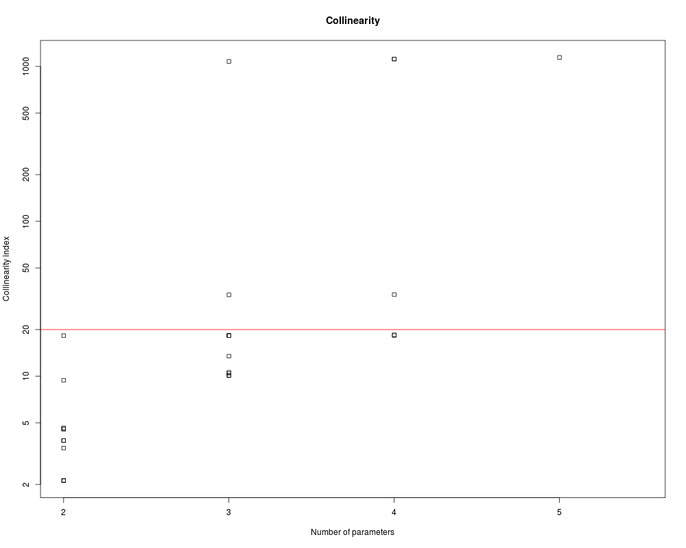
plot(Coll, log = "y")

## 20 = magical number above which there are identifiability problems
abline(h = 20, col = "red")

## select "identifiable" sets with 4 parameters
Coll [Coll[,"collinearity"] < 20 & Coll[,"N"]==4,]

## collinearity of one selected parameter set
collin(sF, c(1, 3, 5))
collin(sF, 1:5)

collin(sF, c("gmax", "eff"))
## collinearity of all combinations of 3 parameters
collin(sF, N = 3)

## The collinearity depends on the value of the parameters:
P      <- pars
P[1:2] <- 1  # was: 0.5
collin(sensFun(Objective, P, varscale = 1))

Results

R version 3.3.1 (2016-06-21) -- "Bug in Your Hair"
Copyright (C) 2016 The R Foundation for Statistical Computing
Platform: x86_64-pc-linux-gnu (64-bit)

R is free software and comes with ABSOLUTELY NO WARRANTY.
You are welcome to redistribute it under certain conditions.
Type 'license()' or 'licence()' for distribution details.

R is a collaborative project with many contributors.
Type 'contributors()' for more information and
'citation()' on how to cite R or R packages in publications.

Type 'demo()' for some demos, 'help()' for on-line help, or
'help.start()' for an HTML browser interface to help.
Type 'q()' to quit R.

> library(FME)
Loading required package: deSolve

Attaching package: 'deSolve'

The following object is masked from 'package:graphics':

    matplot

Loading required package: rootSolve
Loading required package: coda
> png(filename="/home/ddbj/snapshot/RGM3/R_CC/result/FME/collin.Rd_%03d_medium.png", width=480, height=480)
> ### Name: collin
> ### Title: Estimates the Collinearity of Parameter Sets
> ### Aliases: collin plot.collin print.collin
> ### Keywords: utilities
> 
> ### ** Examples
> 
> ## =======================================================================
> ## Test collinearity values
> ## =======================================================================
> 
> ## linearly related set...  => Infinity
> collin(cbind(1:5, 2*(1:5)))
  X1 X2 N collinearity
1  1  1 2          Inf
> 
> ## unrelated set            => 1
> MM <- matrix(nr = 4, nc = 2, byrow = TRUE,
+   data = c(-0.400, -0.374, 0.255, 0.797, 0.690, -0.472, -0.546,  0.049))
> 
> collin(MM)
  X1 X2 N collinearity
1  1  1 2            1
> 
> ## =======================================================================
> ## Bacterial model as in Soetaert and Herman, 2009
> ## =======================================================================
> 
> pars <- list(gmax = 0.5,eff = 0.5,
+              ks = 0.5, rB = 0.01, dB = 0.01)
> 
> solveBact <- function(pars) {
+   derivs <- function(t, state, pars) {   # returns rate of change
+     with (as.list(c(state, pars)), {
+       dBact <-  gmax*eff*Sub/(Sub + ks)*Bact - dB*Bact - rB*Bact
+       dSub  <- -gmax    *Sub/(Sub + ks)*Bact + dB*Bact
+       return(list(c(dBact, dSub)))
+     })
+   }
+   state   <- c(Bact = 0.1, Sub = 100)
+   tout    <- seq(0, 50, by = 0.5)
+   ## ode solves the model by integration...
+   return(as.data.frame(ode(y = state, times = tout, func = derivs,
+     parms = pars)))
+ }
> 
> out <- solveBact(pars)
> 
> ## We wish to estimate parameters gmax and eff by fitting the model to
> ## these data:
> Data <- matrix(nc = 2, byrow = TRUE, data =
+   c(  2,  0.14,  4,  0.2,    6,  0.38,  8,  0.42,
+      10,  0.6,  12,  0.107, 14,  1.3,  16,  2.0,
+      18,  3.0,  20,  4.5,   22,  6.15, 24,  11,
+      26, 13.8,  28, 20.0,   30,  31 ,  35, 65, 40, 61)
+ )
> colnames(Data) <- c("time","Bact")
> head(Data)
     time  Bact
[1,]    2 0.140
[2,]    4 0.200
[3,]    6 0.380
[4,]    8 0.420
[5,]   10 0.600
[6,]   12 0.107
> 
> Data2 <- matrix(c(2, 100, 20, 93, 30, 55, 50, 0), ncol = 2, byrow = TRUE)
> colnames(Data2) <- c("time", "Sub")
> 
> 
> ## Objective function to minimise
> Objective <- function (x) {                  # Model cost
+  pars[] <- x
+  out   <- solveBact(x)
+  Cost  <- modCost(obs = Data2, model = out)  # observed data in 2 data.frames
+  return(modCost(obs = Data, model = out, cost = Cost))
+ }
> 
> ## 1. Estimate sensitivity functions - all parameters
> sF <- sensFun(func = Objective, parms = pars, varscale = 1)
> 
> ## 2. Estimate the collinearity
> Coll <- collin(sF)
> 
> ## The larger the collinearity, the less identifiable the data set
> Coll
   gmax eff ks rB dB N collinearity
1     1   1  0  0  0 2          4.6
2     1   0  1  0  0 2         18.3
3     1   0  0  1  0 2          2.1
4     1   0  0  0  1 2          3.8
5     0   1  1  0  0 2          4.6
6     0   1  0  1  0 2          3.4
7     0   1  0  0  1 2          9.4
8     0   0  1  1  0 2          2.1
9     0   0  1  0  1 2          3.8
10    0   0  0  1  1 2          4.6
11    1   1  1  0  0 3         18.3
12    1   1  0  1  0 3         10.1
13    1   1  0  0  1 3         10.4
14    1   0  1  1  0 3         18.3
15    1   0  1  0  1 3         18.3
16    1   0  0  1  1 3       1077.6
17    0   1  1  1  0 3         10.1
18    0   1  1  0  1 3         10.6
19    0   1  0  1  1 3         13.5
20    0   0  1  1  1 3         33.5
21    1   1  1  1  0 4         18.3
22    1   1  1  0  1 4         18.5
23    1   1  0  1  1 4       1114.9
24    1   0  1  1  1 4       1117.2
25    0   1  1  1  1 4         33.6
26    1   1  1  1  1 5       1143.9
> 
> plot(Coll, log = "y")
> 
> ## 20 = magical number above which there are identifiability problems
> abline(h = 20, col = "red")
> 
> ## select "identifiable" sets with 4 parameters
> Coll [Coll[,"collinearity"] < 20 & Coll[,"N"]==4,]
  gmax eff ks rB dB N collinearity
1    1   1  1  1  0 4           18
2    1   1  1  0  1 4           19
> 
> ## collinearity of one selected parameter set
> collin(sF, c(1, 3, 5))
  gmax eff ks rB dB N collinearity
1    1   0  1  0  1 3           18
> collin(sF, 1:5)
  gmax eff ks rB dB N collinearity
1    1   1  1  1  1 5         1144
> 
> collin(sF, c("gmax", "eff"))
  gmax eff ks rB dB N collinearity
1    1   1  0  0  0 2          4.6
> ## collinearity of all combinations of 3 parameters
> collin(sF, N = 3)
   gmax eff ks rB dB N collinearity
1     1   1  1  0  0 3           18
2     1   1  0  1  0 3           10
3     1   1  0  0  1 3           10
4     1   0  1  1  0 3           18
5     1   0  1  0  1 3           18
6     1   0  0  1  1 3         1078
7     0   1  1  1  0 3           10
8     0   1  1  0  1 3           11
9     0   1  0  1  1 3           13
10    0   0  1  1  1 3           34
> 
> ## The collinearity depends on the value of the parameters:
> P      <- pars
> P[1:2] <- 1  # was: 0.5
> collin(sensFun(Objective, P, varscale = 1))
   gmax eff ks rB dB N collinearity
1     1   1  0  0  0 2          1.3
2     1   0  1  0  0 2        125.6
3     1   0  0  1  0 2          1.0
4     1   0  0  0  1 2        159.9
5     0   1  1  0  0 2          1.3
6     0   1  0  1  0 2          2.1
7     0   1  0  0  1 2          1.3
8     0   0  1  1  0 2          1.0
9     0   0  1  0  1 2        212.4
10    0   0  0  1  1 2          1.0
11    1   1  1  0  0 3        148.8
12    1   1  0  1  0 3          3.3
13    1   1  0  0  1 3        334.2
14    1   0  1  1  0 3        141.2
15    1   0  1  0  1 3        238.3
16    1   0  0  1  1 3        239.7
17    0   1  1  1  0 3          3.3
18    0   1  1  0  1 3        219.9
19    0   1  0  1  1 3          3.3
20    0   0  1  1  1 3        217.6
21    1   1  1  1  0 4        149.0
22    1   1  1  0  1 4        524.2
23    1   1  0  1  1 4        337.5
24    1   0  1  1  1 4        336.5
25    0   1  1  1  1 4        220.0
26    1   1  1  1  1 5        533.0
> 
> 
> 
> 
> 
> 
> dev.off()
null device 
          1 
>