Supported by Dr. Osamu Ogasawara and  . . |
|
Last data update: 2014.03.03 |
Constrained Fitting of a Model to DataDescriptionFitting a model to data, with lower and/or upper bounds UsagemodFit(f, p, ..., lower = -Inf, upper = Inf,
method = c("Marq", "Port", "Newton",
"Nelder-Mead", "BFGS", "CG", "L-BFGS-B", "SANN",
"Pseudo"), jac = NULL,
control = list(), hessian = TRUE)
## S3 method for class 'modFit'
summary(object, cov=TRUE,...)
## S3 method for class 'modFit'
deviance(object, ...)
## S3 method for class 'modFit'
coef(object, ...)
## S3 method for class 'modFit'
residuals(object, ...)
## S3 method for class 'modFit'
df.residual(object, ...)
## S3 method for class 'modFit'
plot(x, ask = NULL, ...)
## S3 method for class 'summary.modFit'
print(x, digits = max(3, getOption("digits") - 3),
...)
Arguments
DetailsNote that arguments after The method to be used is specified by argument
Or one of the following:
For difficult problems it may be efficient to perform some iterations
with The implementation for the routines from In In case both lower and upper bounds are specified, this is achieved by a tangens and arc tangens transformation. This is, parameter values, p', generated by the optimisation
routine, and which are located in the range [-Inf, Inf] are
transformed, before they are passed to p = 1/2 * (upper + lower) + (upper - lower) * arctan(p')/pi . which maps them into the interval [lower, upper]. Before the optimisation routine is called, the original parameter values, as
given by argument p' = tan(pi/2 * (2 * p - upper - lower) / (upper - lower)) In case only lower or upper bounds are specified, this is achieved by a log transformation and a corresponding exponential back transformation. In case parameters are transformed (all methods) or in case the
This ignores the second derivative terms, but this is reasonable if the method has truly converged to the minimum. Note that finite differences are not extremely precise. In case the Levenberg-Marquard method ( Valuea list of class modFit containing the results as returned from the called optimisation routines. This includes the following:
Note: this means that some return arguments of the original optimisation functions are renamed. More specifically, "objective" and "counts" from routine
The list returned by NoteThe The covariance matrix is estimated as 1/(0.5*Hessian). This computation relies on several things, i.e.:
This means that the estimated covariance (correlation) matrix and the confidence intervals derived from it may be worthless if the assumptions behind the covariance computation are invalid. If in doubt about the validity of the summary computations, use Monte Carlo
fitting instead, or run a Other methods included are:
Specifying a function to estimate the Jacobian matrix via argument
Specification of the Author(s)Karline Soetaert <karline.soetaert@nioz.nl>, Thomas Petzoldt <thomas.petzoldt@tu-dresden.de> ReferencesPress, W. H., Teukolsky, S. A., Vetterling, W. T. and Flannery, B. P., 2007. Numerical Recipes in C. Cambridge University Press. Gay, D. M., 1990. Usage Summary for Selected Optimization Routines. Computing Science Technical Report No. 153. AT&T Bell Laboratories, Murray Hill, NJ 07974. http://netlib.bell-labs.com/cm/cs/cstr/153.pdf Soetaert, K. and Petzoldt, T., 2010. Inverse Modelling, Sensitivity and Monte Carlo Analysis in R Using Package FME. Journal of Statistical Software 33(3) 1–28. http://www.jstatsoft.org/v33/i03 See Also
Examples
## =======================================================================
## logistic growth model
## =======================================================================
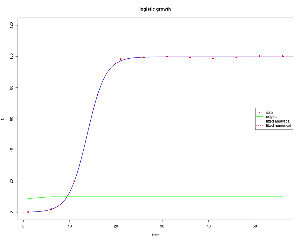
TT <- seq(1, 60, 5)
N0 <- 0.1
r <- 0.5
K <- 100
## perturbed analytical solution
Data <- data.frame(
time = TT,
N = K / (1+(K/N0-1) * exp(-r*TT)) * (1 + rnorm(length(TT), sd = 0.01))
)
plot(TT, Data[,"N"], ylim = c(0, 120), pch = 16, col = "red",
main = "logistic growth", xlab = "time", ylab = "N")
##===================================
## Fitted with analytical solution #
##===================================
## initial "guess"
parms <- c(r = 2, K = 10, N0 = 5)
## analytical solution
model <- function(parms,time)
with (as.list(parms), return(K/(1+(K/N0-1)*exp(-r*time))))
## run the model with initial guess and plot results
lines(TT, model(parms, TT), lwd = 2, col = "green")
## FITTING algorithm 1
ModelCost <- function(P) {
out <- model(P, TT)
return(Data$N-out) # residuals
}
(Fita <- modFit(f = ModelCost, p = parms))
times <- 0:60
lines(times, model(Fita$par, times), lwd = 2, col = "blue")
summary(Fita)
##===================================
## Fitted with numerical solution #
##===================================
## numeric solution
logist <- function(t, x, parms) {
with(as.list(parms), {
dx <- r * x[1] * (1 - x[1]/K)
list(dx)
})
}
## model cost,
ModelCost2 <- function(P) {
out <- ode(y = c(N = P[["N0"]]), func = logist, parms = P, times = c(0, TT))
return(modCost(out, Data)) # object of class modCost
}
Fit <- modFit(f = ModelCost2, p = parms, lower = rep(0, 3),
upper = c(5, 150, 10))
out <- ode(y = c(N = Fit$par[["N0"]]), func = logist, parms = Fit$par,
times = times)
lines(out, col = "red", lty = 2)
legend("right", c("data", "original", "fitted analytical", "fitted numerical"),
lty = c(NA, 1, 1, 2), lwd = c(NA, 2, 2, 1),
col = c("red", "green", "blue", "red"), pch = c(16, NA, NA, NA))
summary(Fit)
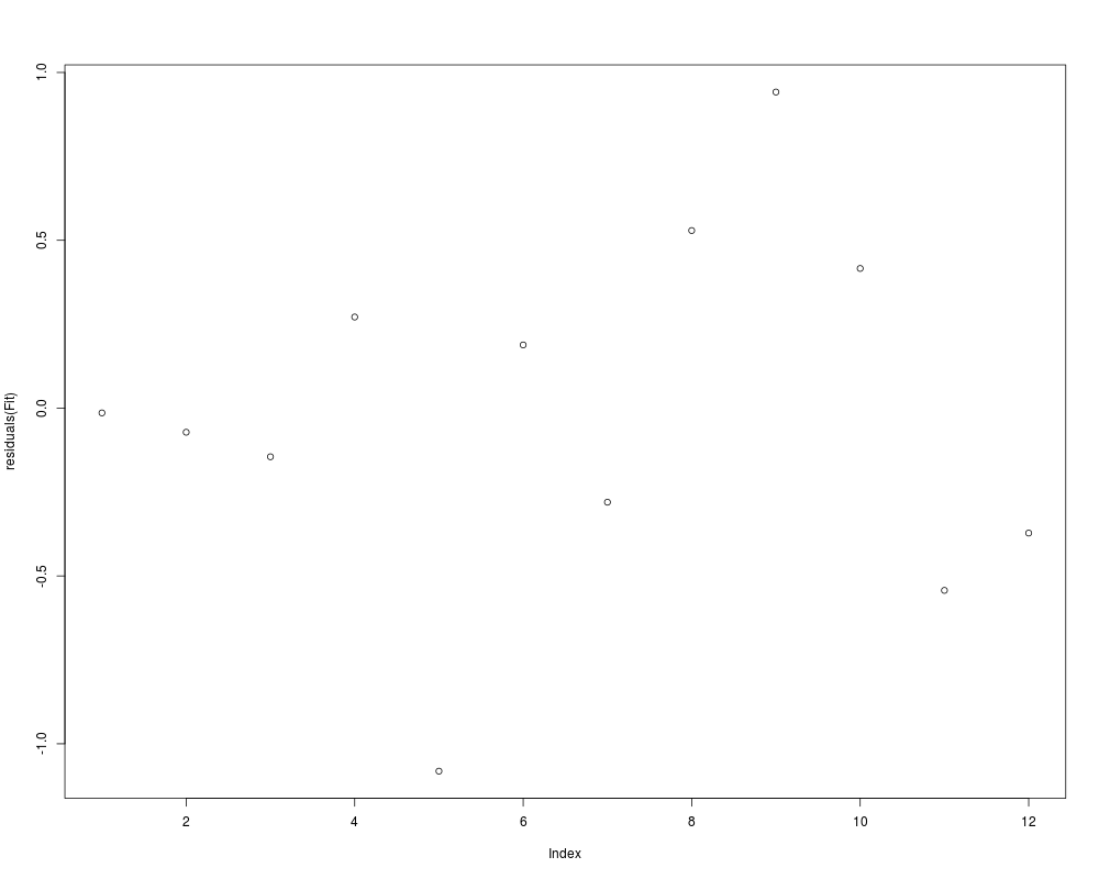
plot(residuals(Fit))
## =======================================================================
## the use of the Jacobian
## =======================================================================
## We use modFit to solve a set of linear equations
A <- matrix(nr = 30, nc = 30, runif(900))
X <- runif(30)
B <- A %*% X
## try to find vector "X"; the Jacobian is matrix A
## Function that returns the vector of residuals
FUN <- function(x)
as.vector(A %*% x - B)
## Function that returns the Jacobian
JAC <- function(x) A
## The port algorithm
print(system.time(
mf <- modFit(f = FUN, p = runif(30), method = "Port")
))
print(system.time(
mf <- modFit(f = FUN, p = runif(30), method = "Port", jac = JAC)
))
max(abs(mf$par - X)) # should be very small
## BFGS
print(system.time(
mf <- modFit(f = FUN, p = runif(30), method = "BFGS")
))
print(system.time(
mf <- modFit(f = FUN, p = runif(30), method = "BFGS", jac = JAC)
))
max(abs(mf$par - X))
## Levenberg-Marquardt
print(system.time(
mf <- modFit(f = FUN, p = runif(30), jac = JAC)
))
max(abs(mf$par - X))
Results
R version 3.3.1 (2016-06-21) -- "Bug in Your Hair"
Copyright (C) 2016 The R Foundation for Statistical Computing
Platform: x86_64-pc-linux-gnu (64-bit)

R is free software and comes with ABSOLUTELY NO WARRANTY.
You are welcome to redistribute it under certain conditions.
Type 'license()' or 'licence()' for distribution details.

R is a collaborative project with many contributors.
Type 'contributors()' for more information and
'citation()' on how to cite R or R packages in publications.

Type 'demo()' for some demos, 'help()' for on-line help, or
'help.start()' for an HTML browser interface to help.
Type 'q()' to quit R.

> library(FME)
Loading required package: deSolve

Attaching package: 'deSolve'

The following object is masked from 'package:graphics':

    matplot

Loading required package: rootSolve
Loading required package: coda
> png(filename="/home/ddbj/snapshot/RGM3/R_CC/result/FME/modFit.Rd_%03d_medium.png", width=480, height=480)
> ### Name: modFit
> ### Title: Constrained Fitting of a Model to Data
> ### Aliases: modFit summary.modFit deviance.modFit coef.modFit
> ###   residuals.modFit df.residual.modFit plot.modFit print.summary.modFit
> ### Keywords: utilities
>
> ### ** Examples
>
>
> ## =======================================================================
> ## logistic growth model
> ## =======================================================================
> TT    <- seq(1, 60, 5)
> N0    <- 0.1
> r     <- 0.5
> K     <- 100
>
> ## perturbed analytical solution
> Data <- data.frame(
+   time = TT,
+      N = K / (1+(K/N0-1) * exp(-r*TT)) * (1 + rnorm(length(TT), sd = 0.01))
+ )
>
> plot(TT, Data[,"N"], ylim = c(0, 120), pch = 16, col = "red",
+      main = "logistic growth", xlab = "time", ylab = "N")
>
>
> ##===================================
> ## Fitted with analytical solution  #
> ##===================================
>
> ## initial "guess"
> parms <- c(r = 2, K = 10, N0 = 5)
>
> ## analytical solution
> model <- function(parms,time)
+   with (as.list(parms), return(K/(1+(K/N0-1)*exp(-r*time))))
>
> ## run the model with initial guess and plot results
> lines(TT, model(parms, TT), lwd = 2, col = "green")
>
> ## FITTING algorithm 1
> ModelCost <- function(P) {
+  out <- model(P, TT)
+  return(Data$N-out)  # residuals
+ }
>
> (Fita <- modFit(f = ModelCost, p = parms))
$par
          r           K          N0
 0.50416083 99.92447333  0.09604409

$hessian
             r         K          N0
r  242446.1347 461.92717 175345.2451
K     461.9272  16.43402    286.4324
N0 175345.2451 286.43244 131340.7844

$residuals
 [1]  0.0042009488  0.0339352047 -0.0041441935  0.0007646018 -0.0345044844
 [6]  0.3068233691  0.4874667626 -0.3161950414 -0.7060947971 -0.4925302094
[11] -0.5510557128  1.3055082584

$info
[1] 1

$message
[1] "Relative error in the sum of squares is at most `ftol'."

$iterations
[1] 22

$rsstrace
 [1] 68704.879822 62600.458874 51433.045799 49667.887390 37748.920845
 [6] 22642.056172  4137.449541  2371.189971   769.622977   632.604506
[11]   472.867211   333.689366   135.753041    98.780053    68.104326
[16]    66.446867    11.138495     8.389125     5.112639     3.947159
[21]     3.183517     3.183291     3.183291

$ssr
[1] 3.183291

$diag
    diag.r     diag.K    diag.N0
698.485317   3.383777 264.529791

$ms
[1] 0.2652743

$var_ms_unscaled
[1] NA

$var_ms_unweighted
[1] NA

$var_ms
[1] NA

$rank
[1] 3

$df.residual
[1] 9

attr(,"class")
[1] "modFit"
>
> times <- 0:60
> lines(times, model(Fita$par, times), lwd = 2, col = "blue")
> summary(Fita)

Parameters:
    Estimate Std. Error t value Pr(>|t|)
r   0.504161   0.009431  53.457 1.41e-12 ***
K  99.924473   0.216786 460.935  < 2e-16 ***
N0  0.096044   0.012710   7.557 3.48e-05 ***
---
Signif. codes:  0 '***' 0.001 '**' 0.01 '*' 0.05 '.' 0.1 ' ' 1

Residual standard error: 0.5947 on 9 degrees of freedom

Parameter correlation:
         r       K      N0
r   1.0000 -0.2188 -0.9825
K  -0.2188  1.0000  0.1796
N0 -0.9825  0.1796  1.0000
>
> ##===================================
> ##  Fitted with numerical solution  #
> ##===================================
>
> ## numeric solution
> logist <- function(t, x, parms) {
+   with(as.list(parms), {
+     dx <- r * x[1] * (1 - x[1]/K)
+     list(dx)
+   })
+ }
>
> ## model cost,
> ModelCost2 <- function(P) {
+  out <- ode(y = c(N = P[["N0"]]), func = logist, parms = P, times = c(0, TT))
+  return(modCost(out, Data))  # object of class modCost
+ }
>
> Fit <- modFit(f = ModelCost2, p = parms, lower = rep(0, 3),
+               upper = c(5, 150, 10))
>
> out <- ode(y = c(N = Fit$par[["N0"]]), func = logist, parms = Fit$par,
+            times = times)
>
> lines(out, col = "red", lty = 2)
> legend("right", c("data", "original", "fitted analytical", "fitted numerical"),
+        lty = c(NA, 1, 1, 2), lwd = c(NA, 2, 2, 1),
+        col = c("red", "green", "blue", "red"), pch = c(16, NA, NA, NA))
> summary(Fit)

Parameters:
    Estimate Std. Error t value Pr(>|t|)
r   0.504161   0.009431  53.457 1.41e-12 ***
K  99.924473   0.216788 460.932  < 2e-16 ***
N0  0.096043   0.012710   7.557 3.48e-05 ***
---
Signif. codes:  0 '***' 0.001 '**' 0.01 '*' 0.05 '.' 0.1 ' ' 1

Residual standard error: 0.5947 on 9 degrees of freedom

Parameter correlation:
         r       K      N0
r   1.0000 -0.2189 -0.9825
K  -0.2189  1.0000  0.1796
N0 -0.9825  0.1796  1.0000
> plot(residuals(Fit))
>
> ## =======================================================================
> ## the use of the Jacobian
> ## =======================================================================
>
> ## We use modFit to solve a set of linear equations
> A <- matrix(nr = 30, nc = 30, runif(900))
> X <- runif(30)
> B <- A %*% X
>
> ## try to find vector "X"; the Jacobian is matrix A
>
> ## Function that returns the vector of residuals
> FUN <- function(x)
+   as.vector(A %*% x - B)
>
> ## Function that returns the Jacobian
> JAC <- function(x) A
>
> ## The port algorithm
> print(system.time(
+   mf <- modFit(f = FUN, p = runif(30), method = "Port")
+ ))
   user  system elapsed
  0.008   0.004   0.013
> print(system.time(
+   mf <- modFit(f = FUN, p = runif(30), method = "Port", jac = JAC)
+ ))
   user  system elapsed
  0.004   0.000   0.003
> max(abs(mf$par - X))  # should be very small
[1] 5.764247e-10
>
> ## BFGS
> print(system.time(
+   mf <- modFit(f = FUN, p = runif(30), method = "BFGS")
+ ))
   user  system elapsed
  0.108   0.000   0.109
> print(system.time(
+   mf <- modFit(f = FUN, p = runif(30), method = "BFGS", jac = JAC)
+ ))
   user  system elapsed
  0.004   0.000   0.003
> max(abs(mf$par - X))
[1] 3.300349e-10
>
> ## Levenberg-Marquardt
> print(system.time(
+   mf <- modFit(f = FUN, p = runif(30), jac = JAC)
+ ))
   user  system elapsed
  0.004   0.000   0.002
> max(abs(mf$par - X))
[1] 4.041212e-14
>
>
>
>
>
> dev.off()
null device
          1
>
|