Supported by Dr. Osamu Ogasawara and  . . |
|
Last data update: 2014.03.03 |
Constrained Markov Chain Monte CarloDescriptionPerforms a Markov Chain Monte Carlo simulation, using an adaptive Metropolis (AM) algorithm and including a delayed rejection (DR) procedure. Usage
modMCMC(f, p, ..., jump = NULL,  lower = -Inf, upper = +Inf,
        prior = NULL, var0 = NULL, wvar0 = NULL, n0 = NULL,
        niter = 1000, outputlength = niter, burninlength = 0,
        updatecov = niter, covscale = 2.4^2/length(p),
        ntrydr = 1, drscale = NULL, verbose = TRUE)


## S3 method for class 'modMCMC'
summary(object, remove = NULL, ...)

## S3 method for class 'modMCMC'
pairs(x, Full = FALSE, which = 1:ncol(x$pars),
  remove = NULL, nsample = NULL, ...)

## S3 method for class 'modMCMC'
hist(x, Full = FALSE, which = 1:ncol(x$pars),
  remove = NULL, ask = NULL, ...)

## S3 method for class 'modMCMC'
plot(x, Full = FALSE, which = 1:ncol(x$pars),
  trace = TRUE, remove = NULL, ask = NULL, ...)
Arguments
DetailsNote that arguments after ... must be matched exactly. R-function In the latter two cases, it is assumed that the prior distribution for theta is either non-informative or gaussian. If gaussian, it can be treated as a sum of squares (SS). If the measurement function is defined as: y = f(p) + xi; xi ~ N(0, sigma^2) where xi is the measurement error, assumed normally distribution, then the posterior for the parameters will be estimated as: prob(p|y,sigma^2)~exp(-0.5 SS(p)/sigma^2)+SSpri(p) and where sigma^2 is the error variance, SS is the sum of squares function SS(p)=sum(yi-f(p))^2. If non-informative priors are used, then SSpri(p)=0. The error variance sigma^2 is considered a nuisance parameter. A prior distribution of it should be specified and a posterior distribution is estimated. If Thus, at each step, 1/ the error variance (sigma^{-2}) is sampled from a gamma distribution: prob(sigma^2|y,p)~Gam(0.5*(n0+n), 0.5*(n0+var0+SS(p)) where The prior parameters ( By setting If If
When When
The jump parameter, If If
Finally, Two methods are implemented to increase the number of accepted runs.
Convergence of the MCMC chain can be checked via In addition, the methods from package The Valuea list of class modMCMC containing the results as returned from the Markov chain. This includes the following:
The list returned by NoteThe following S3 methods are provided:
It is also possible to use the methods from the To do that, first the Author(s)Karline Soetaert <karline.soetaert@nioz.nl> Marko Laine <Marko.Laine@fmi.fi> ReferencesLaine, M., 2008. Adaptive MCMC Methods With Applications in Environmental and Geophysical Models. Finnish Meteorological Institute contributions 69, ISBN 978-951-697-662-7, Finnish Meteorological Institute, Helsinki. Haario, H., Saksman, E. and Tamminen, J., 2001. An Adaptive Metropolis Algorithm. Bernoulli 7, pp. 223–242. Haario, H., Laine, M., Mira, A. and Saksman, E., 2006. DRAM: Efficient Adaptive MCMC. Statistics and Computing, 16(4), 339–354. Haario, H., Saksman, E. and Tamminen, J., 2005. Componentwise Adaptation for High Dimensional MCMC. Computational Statistics 20(2), 265–274. Gelman, A. Varlin, J. B., Stern, H. S. and Rubin, D. B., 2004. Bayesian Data Analysis. Second edition. Chapman and Hall, Boca Raton. Soetaert, K. and Petzoldt, T., 2010. Inverse Modelling, Sensitivity and Monte Carlo Analysis in R Using Package FME. Journal of Statistical Software 33(3) 1–28. http://www.jstatsoft.org/v33/i03 See Also
Examples
## =======================================================================
## Sampling a 3-dimensional normal distribution,
## =======================================================================
# mean = 1:3, sd = 0.1
# f returns -2*log(probability) of the parameter values
NN <- function(p) {
mu <- c(1,2,3)
-2*sum(log(dnorm(p, mean = mu, sd = 0.1))) #-2*log(probability)
}
# simple Metropolis-Hastings
MCMC <- modMCMC(f = NN, p = 0:2, niter = 5000,
outputlength = 1000, jump = 0.5)
# More accepted values by updating the jump covariance matrix...
MCMC <- modMCMC(f = NN, p = 0:2, niter = 5000, updatecov = 100,
outputlength = 1000, jump = 0.5)
summary(MCMC)
plot(MCMC) # check convergence
pairs(MCMC)
## =======================================================================
## test 2: sampling a 3-D normal distribution, larger standard deviation...
## noninformative priors, lower and upper bounds imposed on parameters
## =======================================================================
NN <- function(p) {
mu <- c(1,2,2.5)
-2*sum(log(dnorm(p, mean = mu, sd = 0.5))) #-2*log(probability)
}
MCMC2 <- modMCMC(f = NN, p = 1:3, niter = 2000, burninlength = 500,
updatecov = 10, jump = 0.5, lower = c(0, 2, 1), upper = c(1, 3, 3))
plot(MCMC2)
hist(MCMC2, breaks = 20)
## Compare output of p3 with theoretical distribution
hist(MCMC2, which = "p3", breaks = 20)
lines(seq(1, 3, 0.1), dnorm(seq(1, 3, 0.1), mean = 2.5,
sd = 0.5)/pnorm(3, 2.5, 0.5))
summary(MCMC2)
# functions from package coda...
cumuplot(as.mcmc(MCMC2$pars))
summary(as.mcmc(MCMC2$pars))
raftery.diag(MCMC2$pars)
## =======================================================================
## test 3: sampling a log-normal distribution, log mean=1:4, log sd = 1
## =======================================================================
NL <- function(p) {
mu <- 1:4
-2*sum(log(dlnorm(p, mean = mu, sd = 1))) #-2*log(probability)
}
MCMCl <- modMCMC(f = NL, p = log(1:4), niter = 3000,
outputlength = 1000, jump = 5)
plot(MCMCl) # bad convergence
cumuplot(as.mcmc(MCMCl$pars))
MCMCl <- modMCMC (f = NL, p = log(1:4), niter = 3000,
outputlength = 1000, jump = 2^(2:5))
plot(MCMCl) # better convergence but CHECK it!
pairs(MCMCl)
colMeans(log(MCMCl$pars))
apply(log(MCMCl$pars), 2, sd)
MCMCl <- modMCMC (f = NL, p = rep(1, 4), niter = 3000,
outputlength = 1000, jump = 5, updatecov = 100)
plot(MCMCl)
colMeans(log(MCMCl$pars))
apply(log(MCMCl$pars), 2, sd)
## =======================================================================
## Fitting a Monod (Michaelis-Menten) function to data
## =======================================================================
# the observations
#---------------------
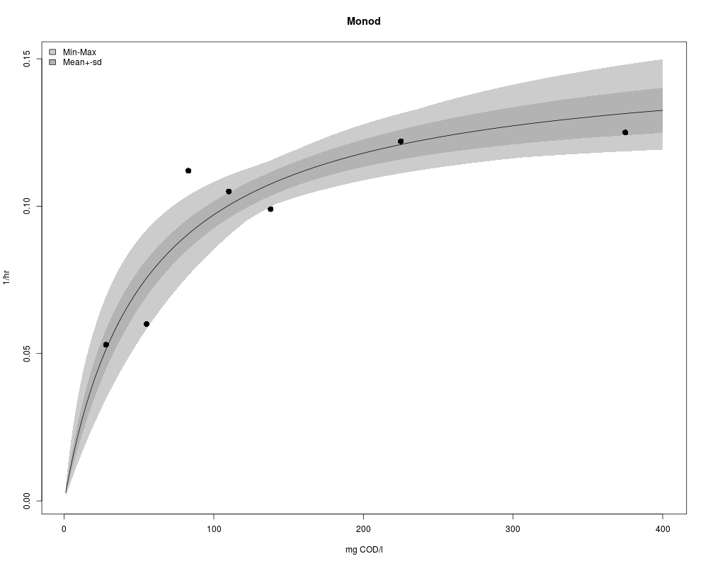
Obs <- data.frame(x=c( 28, 55, 83, 110, 138, 225, 375), # mg COD/l
y=c(0.053,0.06,0.112,0.105,0.099,0.122,0.125)) # 1/hour
plot(Obs, pch = 16, cex = 2, xlim = c(0, 400), ylim = c(0, 0.15),
xlab = "mg COD/l", ylab = "1/hr", main = "Monod")
# the Monod model
#---------------------
Model <- function(p, x) data.frame(x = x, N = p[1]*x/(x+p[2]))
# Fitting the model to the data
#---------------------
# define the residual function
Residuals <- function(p) (Obs$y - Model(p, Obs$x)$N)
# use modFit to find parameters
P <- modFit(f = Residuals, p = c(0.1, 1))
# plot best-fit model
x <-0:375
lines(Model(P$par, x))
# summary of fit
sP <- summary(P)
sP[]
print(sP)
# Running an MCMC
#---------------------
# estimate parameter covariances
# (to efficiently generate new parameter values)
Covar <- sP$cov.scaled * 2.4^2/2
# the model variance
s2prior <- sP$modVariance
# set nprior = 0 to avoid updating model variance
MCMC <- modMCMC(f = Residuals, p = P$par,jump = Covar, niter = 1000,
var0 = s2prior, wvar0 = NULL, updatecov = 100)
plot(MCMC, Full = TRUE)
pairs(MCMC)
# function from the coda package.
raftery.diag(as.mcmc(MCMC$pars))
cor(MCMC$pars)
cov(MCMC$pars) # covariances by MCMC
sP$cov.scaled # covariances by Hessian of fit
x <- 1:400
SR <- summary(sensRange(parInput = MCMC$pars, func = Model, x = x))
plot(SR, xlab="mg COD/l", ylab = "1/hr", main = "Monod")
points(Obs, pch = 16, cex = 1.5)
Results
R version 3.3.1 (2016-06-21) -- "Bug in Your Hair"
Copyright (C) 2016 The R Foundation for Statistical Computing
Platform: x86_64-pc-linux-gnu (64-bit)

R is free software and comes with ABSOLUTELY NO WARRANTY.
You are welcome to redistribute it under certain conditions.
Type 'license()' or 'licence()' for distribution details.

R is a collaborative project with many contributors.
Type 'contributors()' for more information and
'citation()' on how to cite R or R packages in publications.

Type 'demo()' for some demos, 'help()' for on-line help, or
'help.start()' for an HTML browser interface to help.
Type 'q()' to quit R.

> library(FME)
Loading required package: deSolve

Attaching package: 'deSolve'

The following object is masked from 'package:graphics':

    matplot

Loading required package: rootSolve
Loading required package: coda
> png(filename="/home/ddbj/snapshot/RGM3/R_CC/result/FME/modMCMC.Rd_%03d_medium.png", width=480, height=480)
> ### Name: modMCMC
> ### Title: Constrained Markov Chain Monte Carlo
> ### Aliases: modMCMC summary.modMCMC plot.modMCMC pairs.modMCMC
> ###   hist.modMCMC
> ### Keywords: utilities
>
> ### ** Examples
>
>
> ## =======================================================================
> ## Sampling a 3-dimensional normal distribution,
> ## =======================================================================
> # mean = 1:3, sd = 0.1
> # f returns -2*log(probability) of the parameter values
>
> NN <- function(p) {
+   mu <- c(1,2,3)
+   -2*sum(log(dnorm(p, mean = mu, sd = 0.1)))   #-2*log(probability)
+ }
>
> # simple Metropolis-Hastings
> MCMC <- modMCMC(f = NN, p = 0:2, niter = 5000,
+                 outputlength = 1000, jump = 0.5)
number of accepted runs: 134 out of 5000 (2.68%)
>
> # More accepted values by updating the jump covariance matrix...
> MCMC <- modMCMC(f = NN, p = 0:2, niter = 5000, updatecov = 100,
+                  outputlength = 1000, jump = 0.5)
number of accepted runs: 1249 out of 5000 (24.98%)
> summary(MCMC)
            p1        p2        p3
mean 1.0006904 2.0014591 3.0018239
sd   0.1057520 0.1051432 0.1077357
min  0.4945828 1.4837068 2.1677186
max  1.2808472 2.3113110 3.4006987
q025 0.9387839 1.9445865 2.9285290
q050 1.0075769 1.9968258 3.0088521
q075 1.0677240 2.0634510 3.0702421
>
> plot(MCMC)   # check convergence
> pairs(MCMC)
>
> ## =======================================================================
> ## test 2: sampling a 3-D normal distribution, larger standard deviation...
> ## noninformative priors, lower and upper bounds imposed on parameters
> ## =======================================================================
>
> NN <- function(p) {
+   mu <- c(1,2,2.5)
+   -2*sum(log(dnorm(p, mean = mu, sd = 0.5)))   #-2*log(probability)
+ }
>
> MCMC2 <- modMCMC(f = NN, p = 1:3, niter = 2000, burninlength = 500,
+   updatecov = 10, jump = 0.5, lower = c(0, 2, 1), upper = c(1, 3, 3))
number of accepted runs: 572 out of 2000 (28.6%)
> plot(MCMC2)
> hist(MCMC2, breaks = 20)
>
> ## Compare output of p3 with theoretical distribution
> hist(MCMC2, which = "p3", breaks = 20)
> lines(seq(1, 3, 0.1), dnorm(seq(1, 3, 0.1), mean = 2.5,
+   sd = 0.5)/pnorm(3, 2.5, 0.5))
> summary(MCMC2)
             p1        p2        p3
mean 0.58778711 2.3083300 2.3423210
sd   0.25523946 0.2245946 0.4080645
min  0.01217649 2.0016858 1.1530105
max  0.99947918 2.9722593 2.9956495
q025 0.40420642 2.1328337 2.0653973
q050 0.62347823 2.2645638 2.3625641
q075 0.79604275 2.4447484 2.6941603
>
> # functions from package coda...
> cumuplot(as.mcmc(MCMC2$pars))
> summary(as.mcmc(MCMC2$pars))

Iterations = 1:1500
Thinning interval = 1
Number of chains = 1
Sample size per chain = 1500

1. Empirical mean and standard deviation for each variable,
   plus standard error of the mean:

     Mean     SD Naive SE Time-series SE
p1 0.5878 0.2552 0.006590        0.02721
p2 2.3083 0.2246 0.005799        0.01950
p3 2.3423 0.4081 0.010536        0.05081

2. Quantiles for each variable:

      2.5%    25%    50%   75%  97.5%
p1 0.04392 0.4042 0.6235 0.796 0.9824
p2 2.01027 2.1328 2.2646 2.445 2.8174
p3 1.45709 2.0654 2.3626 2.694 2.9566

> raftery.diag(MCMC2$pars)

Quantile (q) = 0.025
Accuracy (r) = +/- 0.005
Probability (s) = 0.95

You need a sample size of at least 3746 with these values of q, r and s
>
> ## =======================================================================
> ## test 3: sampling a log-normal distribution, log mean=1:4, log sd = 1
> ## =======================================================================
>
> NL <- function(p) {
+   mu <- 1:4
+   -2*sum(log(dlnorm(p, mean = mu, sd = 1)))      #-2*log(probability)
+ }
> MCMCl <- modMCMC(f = NL, p = log(1:4), niter = 3000,
+                  outputlength = 1000, jump = 5)
number of accepted runs: 1005 out of 3000 (33.5%)
> plot(MCMCl)   # bad convergence
> cumuplot(as.mcmc(MCMCl$pars))
>
> MCMCl <- modMCMC (f = NL, p = log(1:4), niter = 3000,
+                   outputlength = 1000, jump = 2^(2:5))
number of accepted runs: 723 out of 3000 (24.1%)
> plot(MCMCl)   # better convergence but CHECK it!
> pairs(MCMCl)
> colMeans(log(MCMCl$pars))
      p1       p2       p3       p4
    -Inf 2.225115 2.824419 3.857924
> apply(log(MCMCl$pars), 2, sd)
       p1        p2        p3        p4
      NaN 1.2067198 0.9431331 0.9428958
>
> MCMCl <- modMCMC (f = NL, p = rep(1, 4), niter = 3000,
+                   outputlength = 1000, jump = 5, updatecov = 100)
number of accepted runs: 428 out of 3000 (14.26667%)
> plot(MCMCl)
> colMeans(log(MCMCl$pars))
      p1       p2       p3       p4
1.175229 1.806473 2.976125 3.721921
> apply(log(MCMCl$pars), 2, sd)
       p1        p2        p3        p4
0.9765935 0.8907789 0.9092522 0.9690473
>
> ## =======================================================================
> ## Fitting a Monod (Michaelis-Menten) function to data
> ## =======================================================================
>
> # the observations
> #---------------------
> Obs <- data.frame(x=c(   28,  55,   83,  110,  138,  225,  375),   # mg COD/l
+                   y=c(0.053,0.06,0.112,0.105,0.099,0.122,0.125))   # 1/hour
> plot(Obs, pch = 16, cex = 2, xlim = c(0, 400), ylim = c(0, 0.15),
+      xlab = "mg COD/l", ylab = "1/hr", main = "Monod")
>
> # the Monod model
> #---------------------
> Model <- function(p, x) data.frame(x = x, N = p[1]*x/(x+p[2]))
>
> # Fitting the model to the data
> #---------------------
> # define the residual function
> Residuals  <- function(p) (Obs$y - Model(p, Obs$x)$N)
>
> # use modFit to find parameters
> P      <- modFit(f = Residuals, p = c(0.1, 1))
>
> # plot best-fit model
> x      <-0:375
> lines(Model(P$par, x))
>
> # summary of fit
> sP    <- summary(P)
> sP[]
$residuals
[1]  0.0001564343 -0.0168655247  0.0205985136  0.0044286659 -0.0082846936
[6]  0.0026090929 -0.0035980475

$residualVariance
[1] 0.0001633543

$sigma
[1] 0.01278101

$modVariance
[1] 0.0001166817

$df
[1] 2 5

$cov.unscaled
            [,1]        [,2]
[1,]    1.498016    1531.124
[2,] 1531.123611 1964062.528

$cov.scaled
             [,1]        [,2]
[1,] 0.0002447075   0.2501157
[2,] 0.2501156864 320.8381373

$info
[1] 1

$niter
[1] 6

$stopmess
[1] "ok"

$par
       Estimate  Std. Error  t value     Pr(>|t|)
[1,]  0.1454197  0.01564313 9.296073 0.0002423338
[2,] 49.0529157 17.91195515 2.738557 0.0408620996

> print(sP)

Parameters:
     Estimate Std. Error t value Pr(>|t|)
[1,]  0.14542    0.01564   9.296 0.000242 ***
[2,] 49.05292   17.91196   2.739 0.040862 *
---
Signif. codes:  0 '***' 0.001 '**' 0.01 '*' 0.05 '.' 0.1 ' ' 1

Residual standard error: 0.01278 on 5 degrees of freedom

Parameter correlation:
       [,1]   [,2]
[1,] 1.0000 0.8926
[2,] 0.8926 1.0000
>
> # Running an MCMC
> #---------------------
> # estimate parameter covariances
> # (to efficiently generate new parameter values)
> Covar   <- sP$cov.scaled * 2.4^2/2
>
> # the model variance
> s2prior <- sP$modVariance
>
> # set nprior = 0 to avoid updating model variance
> MCMC <- modMCMC(f = Residuals, p = P$par,jump = Covar, niter = 1000,
+                 var0 = s2prior, wvar0 = NULL, updatecov = 100)
number of accepted runs: 343 out of 1000 (34.3%)
>
> plot(MCMC, Full = TRUE)
> pairs(MCMC)
> # function from the coda package.
> raftery.diag(as.mcmc(MCMC$pars))

Quantile (q) = 0.025
Accuracy (r) = +/- 0.005
Probability (s) = 0.95

You need a sample size of at least 3746 with these values of q, r and s
> cor(MCMC$pars)
          p1        p2
p1 1.0000000 0.9168153
p2 0.9168153 1.0000000
>
> cov(MCMC$pars)   # covariances by MCMC
             p1         p2
p1 0.0002368331   0.263623
p2 0.2636230145 349.108538
> sP$cov.scaled    # covariances by Hessian of fit
             [,1]        [,2]
[1,] 0.0002447075   0.2501157
[2,] 0.2501156864 320.8381373
>
> x  <- 1:400
> SR <- summary(sensRange(parInput = MCMC$pars, func = Model, x = x))
> plot(SR, xlab="mg COD/l", ylab = "1/hr", main = "Monod")
> points(Obs, pch = 16, cex = 1.5)
>
>
>
>
>
>
> dev.off()
null device
          1
>
|