R Graphical Manual

Browse All

Last data update: 2014.03.03

R: Plot Method for observed data

obsplot

R Documentation

Plot Method for observed data

Description

Plot all observed variables in matrix formalt

Usage

obsplot(x, ..., which = NULL, xyswap = FALSE, ask = NULL)

Arguments

`x`	a `matrix` or `data.frame`, containing the observed data to be plotted. The 'x'-values (first axis) should be the first column. Several other matrices or data.frames can be passed in the `...`, after `x` (unnamed) - see second example. If the first column of `x` consists of factors, or characters (strings), then it is assumed that the data are presented in long (database) format, where the first three columns contain (name, x, y). See last example.
`which`	the name(s) or the index to the variables that should be plotted. Default = all variables, except the first column.
`ask`	logical; if `TRUE`, the user is asked before each plot, if `NULL` the user is only asked if more than one page of plots is necessary and the current graphics device is set interactive, see `par(ask=.)` and `dev.interactive`.
`xyswap`	if `TRUE`, then x-and y-values are swapped and the y-axis is from top to bottom. Useful for drawing vertical profiles.
`...`	additional arguments. The graphical arguments are passed to `plot.default` and `points`. The dots may contain other matrices and data.frames with observed data to be plotted on the same graphs as `x` - see second example. The arguments after ... must be matched exactly.

Details

The number of panels per page is automatically determined up to 3 x 3 (par(mfrow = c(3, 3))). This default can be overwritten by specifying user-defined settings for mfrow or mfcol. Set mfrow equal to NULL to avoid the plotting function to change user-defined mfrow or mfcol settings.

Other graphical parameters can be passed as well. Parameters are vectorized, either according to the number of plots (xlab, ylab, main, sub, xlim, ylim, log, asp, ann, axes, frame.plot,panel.first,panel.last, cex.lab,cex.axis,cex.main) or according to the number of lines within one plot (other parameters e.g. col, lty, lwd etc.) so it is possible to assign specific axis labels to individual plots, resp. different plotting style. Plotting parameter ylim, or xlim can also be a list to assign different axis limits to individual plots.

Examples


## 'observed' data
AIRquality <- cbind(DAY = 1:153, airquality[, 1:4])
head(AIRquality)
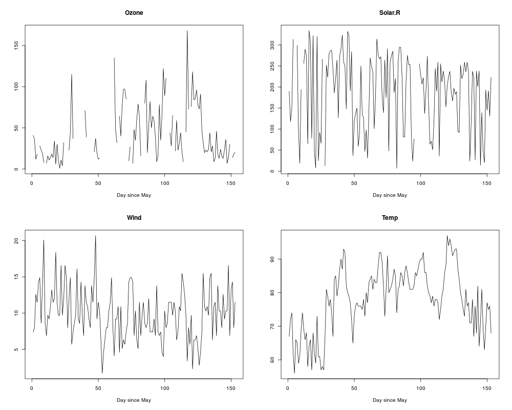
obsplot(AIRquality, type="l", xlab="Day since May")

## second set of observed data
AIR2 <- cbind( 1:100, Solar.R = 250 * runif(100), Temp = 90-30*cos(2*pi*1:100/365) )

obsplot(AIRquality, AIR2, type = "l", xlab = "Day since May" , lwd = 1:2)

obsplot(AIRquality, AIR2, type = "l", xlab = "Day since May" , 
         lwd = 1 : 2, which =c("Solar.R", "Temp"), 
         xlim = list(c(0, 150), c(0, 100)))

obsplot(AIRquality, AIR2, type = "l", xlab = "Day since May" , 
         lwd = 1 : 2, which =c("Solar.R", "Temp"), log = c("y", ""))

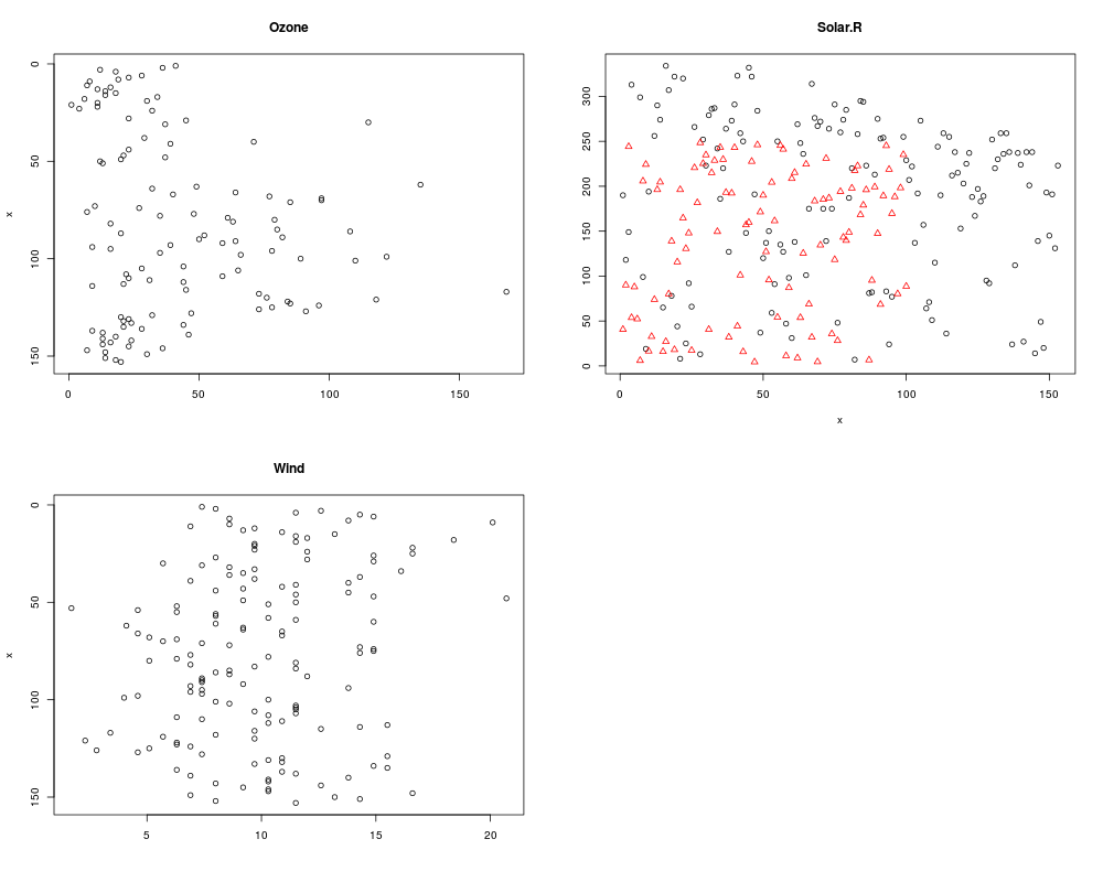
obsplot(AIRquality, AIR2, which = 1:3, xyswap = c(TRUE,FALSE,TRUE))

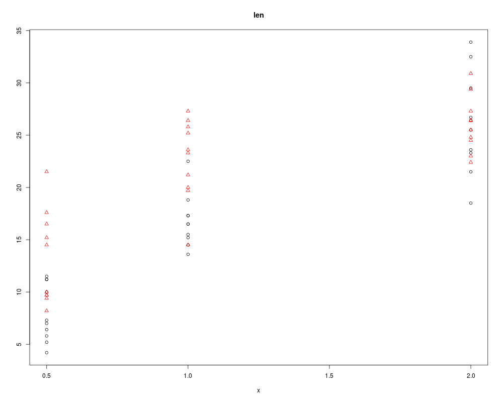
## ' a data.frame, with 'treatments', presented in long database format
Data <- ToothGrowth[,c(2,3,1)]
head   (Data)
obsplot(Data, ylab = "len", xlab = "dose")

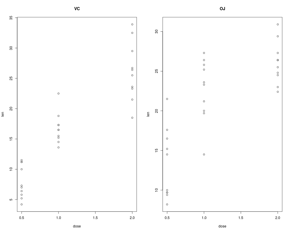
# same, plotted as two observed data sets
obsplot(subset(ToothGrowth, supp == "VC", select = c(dose, len)),
        subset(ToothGrowth, supp == "OJ", select = c(dose, len)))

Results


R version 3.3.1 (2016-06-21) -- "Bug in Your Hair"
Copyright (C) 2016 The R Foundation for Statistical Computing
Platform: x86_64-pc-linux-gnu (64-bit)

R is free software and comes with ABSOLUTELY NO WARRANTY.
You are welcome to redistribute it under certain conditions.
Type 'license()' or 'licence()' for distribution details.

R is a collaborative project with many contributors.
Type 'contributors()' for more information and
'citation()' on how to cite R or R packages in publications.

Type 'demo()' for some demos, 'help()' for on-line help, or
'help.start()' for an HTML browser interface to help.
Type 'q()' to quit R.

> library(FME)
Loading required package: deSolve

Attaching package: 'deSolve'

The following object is masked from 'package:graphics':

    matplot

Loading required package: rootSolve
Loading required package: coda
> png(filename="/home/ddbj/snapshot/RGM3/R_CC/result/FME/obsplot.Rd_%03d_medium.png", width=480, height=480)
> ### Name: obsplot
> ### Title: Plot Method for observed data
> ### Aliases: obsplot
> ### Keywords: hplot
> 
> ### ** Examples
> 
> 
> ## 'observed' data
> AIRquality <- cbind(DAY = 1:153, airquality[, 1:4])
> head(AIRquality)
  DAY Ozone Solar.R Wind Temp
1   1    41     190  7.4   67
2   2    36     118  8.0   72
3   3    12     149 12.6   74
4   4    18     313 11.5   62
5   5    NA      NA 14.3   56
6   6    28      NA 14.9   66
> obsplot(AIRquality, type="l", xlab="Day since May")
> 
> ## second set of observed data
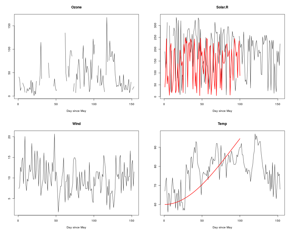
> AIR2 <- cbind( 1:100, Solar.R = 250 * runif(100), Temp = 90-30*cos(2*pi*1:100/365) )
> 
> obsplot(AIRquality, AIR2, type = "l", xlab = "Day since May" , lwd = 1:2)
> 
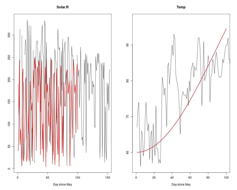
> obsplot(AIRquality, AIR2, type = "l", xlab = "Day since May" , 
+          lwd = 1 : 2, which =c("Solar.R", "Temp"), 
+          xlim = list(c(0, 150), c(0, 100)))
> 
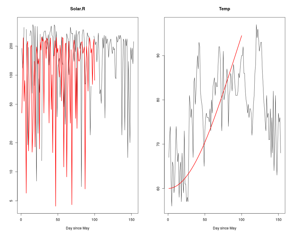
> obsplot(AIRquality, AIR2, type = "l", xlab = "Day since May" , 
+          lwd = 1 : 2, which =c("Solar.R", "Temp"), log = c("y", ""))
> 
> obsplot(AIRquality, AIR2, which = 1:3, xyswap = c(TRUE,FALSE,TRUE))
> 
> ## ' a data.frame, with 'treatments', presented in long database format
> Data <- ToothGrowth[,c(2,3,1)]
> head   (Data)
  supp dose  len
1   VC  0.5  4.2
2   VC  0.5 11.5
3   VC  0.5  7.3
4   VC  0.5  5.8
5   VC  0.5  6.4
6   VC  0.5 10.0
> obsplot(Data, ylab = "len", xlab = "dose")
> 
> # same, plotted as two observed data sets
> obsplot(subset(ToothGrowth, supp == "VC", select = c(dose, len)),
+         subset(ToothGrowth, supp == "OJ", select = c(dose, len)))
> 
> 
> 
> 
> 
> 
> dev.off()
null device 
          1 
>