Supported by Dr. Osamu Ogasawara and  . . |
|
Last data update: 2014.03.03 |
Pseudo-random Search Optimisation Algorithm of Price (1977)DescriptionFits a model to data, using the pseudo-random search algorithm of Price (1977), a random-based fitting technique. UsagepseudoOptim(f, p,..., lower, upper, control = list()) Arguments
DetailsThe
see the book of Soetaert and Herman (2009) for a description of the algorithm AND for a line to line explanation of the function code. Valuea list containing:
and if control$verbose is TRUE:
Author(s)Karline Soetaert <karline.soetaert@nioz.nl> ReferencesSoetaert, K. and Herman, P. M. J., 2009. A Practical Guide to Ecological Modelling. Using R as a Simulation Platform. Springer, 372 pp. Price, W.L., 1977. A Controlled Random Search Procedure for Global Optimisation. The Computer Journal, 20: 367-370. Examples
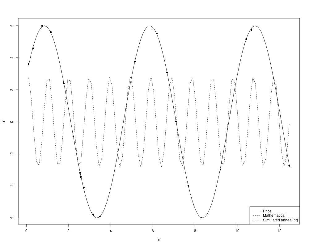
amp    <- 6
period <- 5
phase  <- 0.5

x <- runif(20)*13
y <- amp*sin(2*pi*x/period+phase) + rnorm(20, mean = 0, sd = 0.05)
plot(x, y, pch = 16)


cost <- function(par)
    sum((par[1] * sin(2*pi*x/par[2]+par[3])-y)^2)

p1 <- optim(par = c(amplitude = 1, phase = 1, period = 1), fn = cost)
p2 <- optim(par = c(amplitude = 1, phase = 1, period = 1), fn = cost,
            method = "SANN")
p3 <- pseudoOptim(p = c(amplitude = 1, phase = 1, period = 1),
            lower = c(0, 1e-8, 0), upper = c(100, 2*pi, 100),
            f = cost, control = c(numiter = 3000, verbose = TRUE))

curve(p1$par[1]*sin(2*pi*x/p1$par[2]+p1$par[3]), lty = 2, add = TRUE)
curve(p2$par[1]*sin(2*pi*x/p2$par[2]+p2$par[3]), lty = 3, add = TRUE)
curve(p3$par[1]*sin(2*pi*x/p3$par[2]+p3$par[3]), lty = 1, add = TRUE)
legend ("bottomright", lty = c(1, 2, 3),
         c("Price", "Mathematical", "Simulated annealing"))
Results
R version 3.3.1 (2016-06-21) -- "Bug in Your Hair"
Copyright (C) 2016 The R Foundation for Statistical Computing
Platform: x86_64-pc-linux-gnu (64-bit)

R is free software and comes with ABSOLUTELY NO WARRANTY.
You are welcome to redistribute it under certain conditions.
Type 'license()' or 'licence()' for distribution details.

R is a collaborative project with many contributors.
Type 'contributors()' for more information and
'citation()' on how to cite R or R packages in publications.

Type 'demo()' for some demos, 'help()' for on-line help, or
'help.start()' for an HTML browser interface to help.
Type 'q()' to quit R.

> library(FME)
Loading required package: deSolve

Attaching package: 'deSolve'

The following object is masked from 'package:graphics':

    matplot

Loading required package: rootSolve
Loading required package: coda
> png(filename="/home/ddbj/snapshot/RGM3/R_CC/result/FME/pseudoOptim.Rd_%03d_medium.png", width=480, height=480)
> ### Name: pseudoOptim
> ### Title: Pseudo-random Search Optimisation Algorithm of Price (1977)
> ### Aliases: pseudoOptim
> ### Keywords: optimize
>
> ### ** Examples
>
> amp    <- 6
> period <- 5
> phase  <- 0.5
>
> x <- runif(20)*13
> y <- amp*sin(2*pi*x/period+phase) + rnorm(20, mean = 0, sd = 0.05)
> plot(x, y, pch = 16)
>
>
> cost <- function(par)
+     sum((par[1] * sin(2*pi*x/par[2]+par[3])-y)^2)
>
> p1 <- optim(par = c(amplitude = 1, phase = 1, period = 1), fn = cost)
> p2 <- optim(par = c(amplitude = 1, phase = 1, period = 1), fn = cost,
+             method = "SANN")
> p3 <- pseudoOptim(p = c(amplitude = 1, phase = 1, period = 1),
+             lower = c(0, 1e-8, 0), upper = c(100, 2*pi, 100),
+             f = cost, control = c(numiter = 3000, verbose = TRUE))
>
> curve(p1$par[1]*sin(2*pi*x/p1$par[2]+p1$par[3]), lty = 2, add = TRUE)
> curve(p2$par[1]*sin(2*pi*x/p2$par[2]+p2$par[3]), lty = 3, add = TRUE)
> curve(p3$par[1]*sin(2*pi*x/p3$par[2]+p3$par[3]), lty = 1, add = TRUE)
> legend ("bottomright", lty = c(1, 2, 3),
+          c("Price", "Mathematical", "Simulated annealing"))
>
>
>
>
> dev.off()
null device
          1
>
|