R Graphical Manual

Browse All

Last data update: 2014.03.03

R: Computes the Leslie or Delury population estimate from catch...

depletion

R Documentation

Computes the Leslie or Delury population estimate from catch and effort data.

Description

Computes the Leslie or Delury estimates of population size and catchability coefficient from paired catch and effort data. The Ricker modification may also be used.

Usage

depletion(catch, effort, method = c("Leslie", "DeLury", "Delury"),
  Ricker.mod = FALSE)

## S3 method for class 'depletion'
summary(object, type = c("params", "lm"),
  verbose = FALSE, digits = getOption("digits"), ...)

## S3 method for class 'depletion'
coef(object, type = c("params", "lm"),
  digits = getOption("digits"), ...)

## S3 method for class 'depletion'
confint(object, parm = c("No", "q", "lm"),
  level = conf.level, conf.level = 0.95, digits = getOption("digits"),
  ...)

## S3 method for class 'depletion'
anova(object, ...)

## S3 method for class 'depletion'
plot(x, xlab = NULL, ylab = NULL, pch = 19,
  col.pt = "black", col.mdl = "gray70", lwd = 1, lty = 1,
  pos.est = "topright", cex.est = 0.95, ...)

Arguments

`catch`	A numeric vector of catches of fish at each time.
`effort`	A numeric vector of efforts expended at each time.
`method`	A single string that indicates which depletion method to use
`Ricker.mod`	A single logical that indicates whether to use the modification proposed by Ricker (=TRUE) or not (=FALSE, default).
`object`	An object saved from the `removal` call (i.e., of class `depletion`).
`type`	A string that indicates the type of summary or coefficients to extract. If `type="params"` (the default) then results for No and q are returned. If `type="lm"` then results for the underlying linear model are returned.
`verbose`	A logical that indicates whether a reminder of the method used should be printed with the summary results.
`digits`	A single numeric indicating the number of digits to round the output.
`parm`	A specification of which parameters are to be given confidence intervals, either a vector of numbers or a vector of names. If missing, all parameters are considered.
`level`	Same as `conf.level` but used for compatability with generic `confint` function.
`conf.level`	A single number that represents the level of confidence to use for constructing confidence intervals.
`x`	An object saved from the `depletion` call (i.e., of class `depletion`).
`xlab`	A label for the x-axis.
`ylab`	A label for the y-axis.
`pch`	A numeric that indicates the type of plotting character.
`col.pt`	A string that indicates the color of the plotted points.
`col.mdl`	A string that indicates the color of the fitted line.
`lwd`	A numeric that indicates the line width of the fitted line.
`lty`	A numeric that indicates the type of line used for the fitted line.
`pos.est`	A single string to identify where to place the estimated population estimate and catchability on the plot. Can be set to one of `"bottomright"`, `"bottom"`, `"bottomleft"`, `"left"`, `"topleft"`, `"top"`, `"topright"`, `"right"` or `"center"` for positioning the estimated mortality rates on the plot. Typically `"bottomleft"` (DEFAULT) and `"topright"` will be “out-of-the-way” placements. Set `pos.est` to `NULL` to remove the estimated population size and catchability coefficient from the plot.
`cex.est`	A single numeric that identifies the character expansion value for the estimated population estimate and catchability placed on the plot.
`...`	Additional arguments for methods.

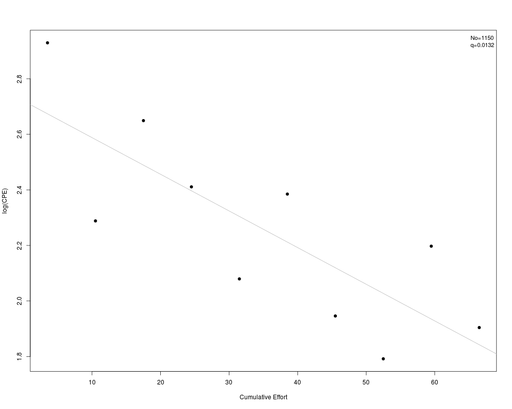
Details

For the Leslie method, a linear regression model of catch-per-unit-effort on cumulative catch prior to the sample is fit. The catchability coefficient (q) is estimated from the negative of the slope and the initial population size (No) is estimated by dividing the intercept by the catchability coefficient. If Ricker.mod=TRUE then the cumulative catch is modified to be the cumulative catch prior to the sample plus half of the catch of the current sample.

For the DeLury method, a linear regression model of log (catch-per-unit-effort) on cumulative effort is fit. The catchability coefficient (q) is estimated from the negative of the slope and the initial population size (No) is estimated by dividing the intercept as an exponent of e by the catchability coefficient. If Ricker.mod=TRUE then the cumulative effort is modified to be the cumulative effort prior to the sample plus half of the effort of the current sample.

Standard errors for the catchability and population size estimates are computed fronm formulas on page 298 (for Leslie) and 303 (for DeLury) from Seber (2002). Confidence intervals are computed using standard large-sample normal distribution theory with the regression error df.

Value

A list with the following items:

method A string that indicates whether the "Leslie" or "Delury" model was used.
catch The original vector of catches.
effort The orginal vector of efforts.
cpe A computed vector of catch-per-unit-effort for each time.
KorE A computed vector of cumulative catch (K; Leslie method) or effort (E; Delury method).
lm The lm object from the fit of CPE on K (Leslie method) or log(CPE) on E (Delury method).
est A 2x2 matrix that contains the estimates and standard errors for No and q.

testing

The Leslie method without the Ricker modification and the DeLury method with the Ricker modification matches the results from deplet in fishmethods for the darter (from fishmethods), LobsterPEI and BlueCrab from FSAdata, and SMBassLS for N0 to whole numbers, the SE for No to one decimal, q to seven decimals, and the SE of q to at least five decimals.

The Leslie method matches the results of Seber (2002) for N0, q, and the CI for Q but not the CI for N (which was so far off that it might be that Seber's result is incorrect) for the lobster data and the q and CI for q but the NO or its CI (likely due to lots of rounding in Seber 2002) for the Blue Crab data.

The Leslie and DeLury methods match the results of Ricker (1975) for No and Q but not for the CI of No (Ricker used a very different method to compute CIs).

IFAR Chapter

10-Abundance from Depletion Data.

Author(s)

Derek H. Ogle, derek@derekogle.com

References

Ogle, D.H. 2016. Introductory Fisheries Analyses with R. Chapman & Hall/CRC, Boca Raton, FL.

Ricker, W.E. 1975. Computation and interpretation of biological statistics of fish populations. Technical Report Bulletin 191, Bulletin of the Fisheries Research Board of Canada. [Was (is?) from http://www.dfo-mpo.gc.ca/Library/1485.pdf.]

Seber, G.A.F. 2002. The Estimation of Animal Abundance. Edward Arnold, Second edition (reprinted).

Examples

data(SMBassLS)

## Leslie model examples
# no Ricker modification
l1 <- depletion(SMBassLS$catch,SMBassLS$effort,method="Leslie")
coef(l1)
summary(l1)
summary(l1,verbose=TRUE)
confint(l1)
summary(l1,type="lm")
plot(l1)

# with Ricker modification
l2 <- depletion(SMBassLS$catch,SMBassLS$effort,method="Leslie",Ricker.mod=TRUE)
summary(l2)
confint(l2)
plot(l2)

## Delury model examples
# no Ricker modification
d1 <- depletion(SMBassLS$catch,SMBassLS$effort,method="Delury")
coef(d1)
summary(d1)
summary(d1,verbose=TRUE)
confint(d1)
summary(d1,type="lm")
plot(d1)

# with Ricker modification
d2 <- depletion(SMBassLS$catch,SMBassLS$effort,method="Delury",Ricker.mod=TRUE)
summary(d2)
confint(d2)
plot(d2)

Results


R version 3.3.1 (2016-06-21) -- "Bug in Your Hair"
Copyright (C) 2016 The R Foundation for Statistical Computing
Platform: x86_64-pc-linux-gnu (64-bit)

R is free software and comes with ABSOLUTELY NO WARRANTY.
You are welcome to redistribute it under certain conditions.
Type 'license()' or 'licence()' for distribution details.

R is a collaborative project with many contributors.
Type 'contributors()' for more information and
'citation()' on how to cite R or R packages in publications.

Type 'demo()' for some demos, 'help()' for on-line help, or
'help.start()' for an HTML browser interface to help.
Type 'q()' to quit R.

> library(FSA)


 ############################################
 ##      FSA package, version 0.8.7        ##
 ##    Derek H. Ogle, Northland College    ##
 ##                                        ##
 ## Run ?FSA for documentation.            ##
 ## Run citation('FSA') for citation ...   ##
 ##   please cite if used in publication.  ##
 ##                                        ##
 ## See derekogle.com/fishR/ for more      ##
 ##   thorough analytical vignettes.       ##
 ############################################


> png(filename="/home/ddbj/snapshot/RGM3/R_CC/result/FSA/depletion.Rd_%03d_medium.png", width=480, height=480)
> ### Name: depletion
> ### Title: Computes the Leslie or Delury population estimate from catch and
> ###   effort data.
> ### Aliases: anova.depletion coef.depletion confint.depletion depletion
> ###   plot.depletion summary.depletion
> ### Keywords: hplot manip
> 
> ### ** Examples
> 
> data(SMBassLS)
> 
> ## Leslie model examples
> # no Ricker modification
> l1 <- depletion(SMBassLS$catch,SMBassLS$effort,method="Leslie")
> coef(l1)
           No        q
[1,] 1060.296 0.014844
> summary(l1)
      Estimate   Std. Err.
No 1060.295599 169.2676197
q     0.014844   0.0035205
> summary(l1,verbose=TRUE)
The Leslie method was used.
      Estimate   Std. Err.
No 1060.295599 169.2676197
q     0.014844   0.0035205
> confint(l1)
       95% LCI      95% UCI
No 669.9637682 1450.6274302
q    0.0067257    0.0229623
> summary(l1,type="lm")

Call:
stats::lm(formula = cpe ~ K)

Residuals:
    Min      1Q  Median      3Q     Max 
-3.9373 -1.3879  0.3295  1.5023  2.9752 

Coefficients:
            Estimate Std. Error t value Pr(>|t|)    
(Intercept) 15.73906    1.51266  10.405 6.31e-06 ***
K           -0.01484    0.00352  -4.216  0.00293 ** 
---
Signif. codes:  0 '***' 0.001 '**' 0.01 '*' 0.05 '.' 0.1 ' ' 1

Residual standard error: 2.295 on 8 degrees of freedom
Multiple R-squared:  0.6897,	Adjusted R-squared:  0.6509 
F-statistic: 17.78 on 1 and 8 DF,  p-value: 0.00293

> plot(l1)
> 
> # with Ricker modification
> l2 <- depletion(SMBassLS$catch,SMBassLS$effort,method="Leslie",Ricker.mod=TRUE)
> summary(l2)
       Estimate   Std. Err.
No 1077.5713043 177.8035211
q     0.0152508   0.0039116
> confint(l2)
       95% LCI     95% UCI
No 667.5556494 1487.586959
q    0.0062306    0.024271
> plot(l2)
> 
> ## Delury model examples
> # no Ricker modification
> d1 <- depletion(SMBassLS$catch,SMBassLS$effort,method="Delury")
> coef(d1)
           No         q
[1,] 1098.503 0.0131938
> summary(d1)
       Estimate   Std. Err.
No 1098.5032552 191.6048926
q     0.0131938   0.0035858
> summary(d1,verbose=TRUE)
The DeLury method was used.
       Estimate   Std. Err.
No 1098.5032552 191.6048926
q     0.0131938   0.0035858
> confint(d1)
       95% LCI      95% UCI
No 656.6615805 1540.3449299
q    0.0049249    0.0214627
> summary(d1,type="lm")

Call:
stats::lm(formula = log(cpe) ~ E)

Residuals:
     Min       1Q   Median       3Q      Max 
-0.29314 -0.21203  0.03796  0.16974  0.26238 

Coefficients:
             Estimate Std. Error t value Pr(>|t|)    
(Intercept)  2.673692   0.134000  19.953 4.15e-08 ***
E           -0.013194   0.003586  -3.679  0.00622 ** 
---
Signif. codes:  0 '***' 0.001 '**' 0.01 '*' 0.05 '.' 0.1 ' ' 1

Residual standard error: 0.228 on 8 degrees of freedom
Multiple R-squared:  0.6286,	Adjusted R-squared:  0.5821 
F-statistic: 13.54 on 1 and 8 DF,  p-value: 0.006224

> plot(d1)
> 
> # with Ricker modification
> d2 <- depletion(SMBassLS$catch,SMBassLS$effort,method="Delury",Ricker.mod=TRUE)
> summary(d2)
      Estimate   Std. Err.
No 1.15042e+03 187.6083109
q  1.31938e-02   0.0035858
> confint(d2)
       95% LCI      95% UCI
No 717.7940216 1583.0451030
q    0.0049249    0.0214627
> plot(d2)
> 
> 
> 
> 
> 
> 
> dev.off()
null device 
          1 
>