R Graphical Manual

Browse All

Last data update: 2014.03.03

R: Find reasonable starting values for a von Bertalanffy growth...

vbStarts

R Documentation

Find reasonable starting values for a von Bertalanffy growth function.

Description

Finds reasonable starting values for the parameters in a specific parameterization of the von Bertalanffy growth function.

Usage

vbStarts(formula, data = NULL, param = c("Typical", "typical",
  "Traditional", "traditional", "BevertonHolt", "Original", "original",
  "vonBertalanffy", "GQ", "GallucciQuinn", "Mooij", "Weisberg", "Schnute",
  "Francis", "Somers", "Somers2"), type = param, ages2use = NULL,
  methEV = c("means", "poly"), meth0 = c("yngAge", "poly"), plot = FALSE,
  col.mdl = "gray70", lwd.mdl = 3, lty.mdl = 1, cex.main = 0.9,
  col.main = "red", dynamicPlot = FALSE, ...)

Arguments

`formula`	A formula of the form `len~age`.
`data`	A data frame that contains the variables in `formula`.
`type, param`	A string that indicates the parameterization of the von Bertalanffy model.
`ages2use`	A numerical vector of the two ages to be used in the Schnute or Francis paramaterizations. See details.
`methEV`	A string that indicates how the lengths of the two ages in the Schnute paramaterization or the three ages in the Francis paramaterization should be derived. See details.
`meth0`	A string that indicates how the t0 and L0 paramaters should be derived. See details.
`plot`	A logical that indicates whether a plot of the data with the superimposed model fit at the starting values should be created.
`col.mdl`	A color for the model when `plot=TRUE`.
`lwd.mdl`	A line width for the model when `plot=TRUE`.
`lty.mdl`	A line type for the model when `plot=TRUE`.
`cex.main`	A character expansion value for the main title when `plot=TRUE`.
`col.main`	A color for the main title when `plot=TRUE`.
`dynamicPlot`	DEPRECATED.
`...`	Further arguments passed to the methods.

Details

This function attempts to find reasonable starting values for a variety of parameterizations of the von Bertalanffy growth function. There is no guarantee that these starting values are the ‘best’ starting values. One should use them with caution and should perform sensitivity analyses to determine the impact of different starting values on the final model results.

The Linf and K paramaters are estimated via the concept of the Ford-Walford plot. The product of the starting values for Linf and K is used as a starting value for omega in the GallucciQuinn and Mooij parameterizations. The result of log(2) divided by the starting value for K is used as the starting value for t50 in the Weisberg parameterization.

If meth0="yngAge", then a starting value for t0 or L0 is found by algebraically solving the typical or original paramaterization, respectively, for t0 or L0 using the mean length of the first age with more than one data point as a “known” quantity. If meth0="poly" then a second-degree polynomial model is fit to the mean length-at-age data. The t0 starting value is set equal to the root of the polynomial that is closest to zero. The L0 starting value is set equal to the mean length at age-0 predicted from the polynomial function.

Starting values for the L1 and L3 parameters in the Schnute paramaterization and the L1, L2, and L3 parameters in the Francis parameterization may be found in two ways. If methEV="poly", then the starting values are the predicted length-at-age from a second-degree polynomial fit to the mean lengths-at-age data. If methEV="means" then the observed sample means at the corresponding ages are used. In the case where one of the supplied ages is fractional, then the value returned will be linearly interpolated between the mean lengths of the two closest ages. The ages to be used for L1 and L3 in the Schnute and Francis parameterizations are supplied as a numeric vector of length 2 in ages2use=. If ages2use=NULL then the minimum and maximum observed ages will be used. In the Francis method, L2 will correspond to the age half-way between the two ages in ages2use=. A warning will be given if L2<L1 for the Schnute method or if L2<L1 or L3<L2 for the Francis method.

Value

A list that contains reasonable starting values. Note that the parameters will be listed in the same order and with the same names as listed in vbFuns.

IFAR Chapter

12-Individual Growth.

Note

The ‘original’ and ‘vonBertalanffy’ and the ‘typical’ and ‘BevertonHolt’ parameterizations are synonymous.

Author(s)

Derek H. Ogle, derek@derekogle.com

References

Ogle, D.H. 2016. Introductory Fisheries Analyses with R. Chapman & Hall/CRC, Boca Raton, FL.

See references in vbFuns.

Examples

## Examples
data(SpotVA1)
vbStarts(tl~age,data=SpotVA1)
vbStarts(tl~age,data=SpotVA1,type="Original")
vbStarts(tl~age,data=SpotVA1,type="GQ")
vbStarts(tl~age,data=SpotVA1,type="Mooij")
vbStarts(tl~age,data=SpotVA1,type="Weisberg")
vbStarts(tl~age,data=SpotVA1,type="Francis",ages2use=c(0,5))
vbStarts(tl~age,data=SpotVA1,type="Schnute",ages2use=c(0,5))
vbStarts(tl~age,data=SpotVA1,type="Somers")
vbStarts(tl~age,data=SpotVA1,type="Somers2")

## Using a different method to find t0 and L0
vbStarts(tl~age,data=SpotVA1,meth0="yngAge")
vbStarts(tl~age,data=SpotVA1,type="original",meth0="yngAge")

## Using a different method to find the L1, L2, and L3
vbStarts(tl~age,data=SpotVA1,type="Francis",ages2use=c(0,5),methEV="means")
vbStarts(tl~age,data=SpotVA1,type="Schnute",ages2use=c(0,5),methEV="means")

## Example with a Plot
vbStarts(tl~age,data=SpotVA1,plot=TRUE)
vbStarts(tl~age,data=SpotVA1,type="original",plot=TRUE)
vbStarts(tl~age,data=SpotVA1,type="GQ",plot=TRUE)
vbStarts(tl~age,data=SpotVA1,type="Mooij",plot=TRUE)
vbStarts(tl~age,data=SpotVA1,type="Weisberg",plot=TRUE)
vbStarts(tl~age,data=SpotVA1,type="Francis",ages2use=c(0,5),plot=TRUE)
vbStarts(tl~age,data=SpotVA1,type="Schnute",ages2use=c(0,5),plot=TRUE)
vbStarts(tl~age,data=SpotVA1,type="Somers",plot=TRUE)
vbStarts(tl~age,data=SpotVA1,type="Somers2",plot=TRUE)

## See examples in vbFuns() for use of vbStarts() when fitting Von B models

Results


R version 3.3.1 (2016-06-21) -- "Bug in Your Hair"
Copyright (C) 2016 The R Foundation for Statistical Computing
Platform: x86_64-pc-linux-gnu (64-bit)

R is free software and comes with ABSOLUTELY NO WARRANTY.
You are welcome to redistribute it under certain conditions.
Type 'license()' or 'licence()' for distribution details.

R is a collaborative project with many contributors.
Type 'contributors()' for more information and
'citation()' on how to cite R or R packages in publications.

Type 'demo()' for some demos, 'help()' for on-line help, or
'help.start()' for an HTML browser interface to help.
Type 'q()' to quit R.

> library(FSA)


 ############################################
 ##      FSA package, version 0.8.7        ##
 ##    Derek H. Ogle, Northland College    ##
 ##                                        ##
 ## Run ?FSA for documentation.            ##
 ## Run citation('FSA') for citation ...   ##
 ##   please cite if used in publication.  ##
 ##                                        ##
 ## See derekogle.com/fishR/ for more      ##
 ##   thorough analytical vignettes.       ##
 ############################################


> png(filename="/home/ddbj/snapshot/RGM3/R_CC/result/FSA/vbStarts.Rd_%03d_medium.png", width=480, height=480)
> ### Name: vbStarts
> ### Title: Find reasonable starting values for a von Bertalanffy growth
> ###   function.
> ### Aliases: vbStarts
> ### Keywords: manip
> 
> ### ** Examples
> 
> ## Examples
> data(SpotVA1)
> vbStarts(tl~age,data=SpotVA1)
$Linf
[1] 13.26773

$K
[1] 0.4114688

$t0
[1] -2.124367

> vbStarts(tl~age,data=SpotVA1,type="Original")
$Linf
[1] 13.26773

$L0
[1] 7.732

$K
[1] 0.4114688

> vbStarts(tl~age,data=SpotVA1,type="GQ")
$omega
[1] 5.459258

$K
[1] 0.4114688

$t0
[1] -2.124367

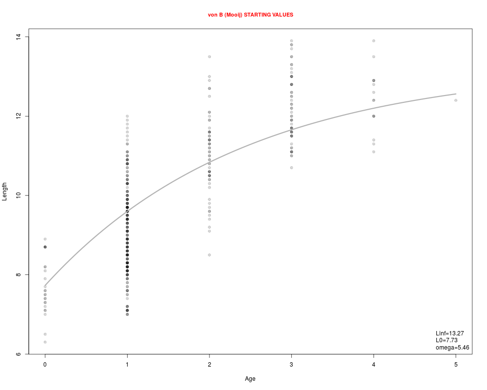
> vbStarts(tl~age,data=SpotVA1,type="Mooij")
$Linf
[1] 13.26773

$L0
[1] 7.732

$omega
[1] 5.459258

> vbStarts(tl~age,data=SpotVA1,type="Weisberg")
$Linf
[1] 13.26773

$t50
[1] -0.4397993

$t0
[1] -2.124367

> vbStarts(tl~age,data=SpotVA1,type="Francis",ages2use=c(0,5))
$L1
[1] 7.732

$L2
[1] 11.60785

$L3
[1] 12.4

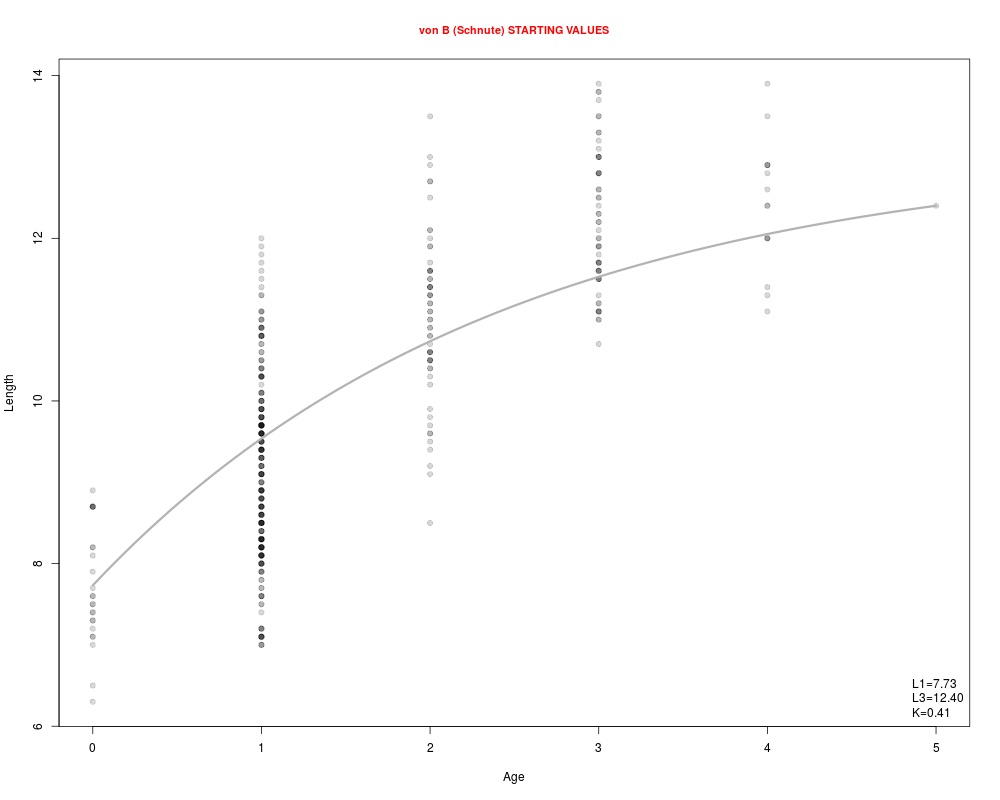
> vbStarts(tl~age,data=SpotVA1,type="Schnute",ages2use=c(0,5))
$L1
[1] 7.732

$L3
[1] 12.4

$K
[1] 0.4114688

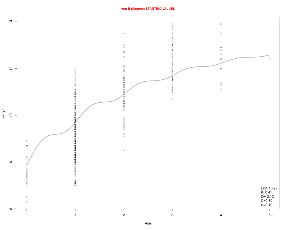
> vbStarts(tl~age,data=SpotVA1,type="Somers")
$Linf
[1] 13.26773

$K
[1] 0.4114688

$t0
[1] -2.124367

$C
[1] 0.9

$ts
[1] 0.1

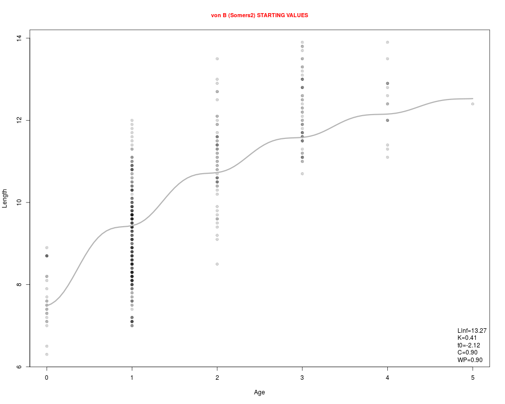
> vbStarts(tl~age,data=SpotVA1,type="Somers2")
$Linf
[1] 13.26773

$K
[1] 0.4114688

$t0
[1] -2.124367

$C
[1] 0.9

$WP
[1] 0.9

> 
> ## Using a different method to find t0 and L0
> vbStarts(tl~age,data=SpotVA1,meth0="yngAge")
$Linf
[1] 13.26773

$K
[1] 0.4114688

$t0
[1] -2.124367

> vbStarts(tl~age,data=SpotVA1,type="original",meth0="yngAge")
$Linf
[1] 13.26773

$L0
[1] 7.732

$K
[1] 0.4114688

> 
> ## Using a different method to find the L1, L2, and L3
> vbStarts(tl~age,data=SpotVA1,type="Francis",ages2use=c(0,5),methEV="means")
$L1
[1] 7.732

$L2
[1] 11.60785

$L3
[1] 12.4

> vbStarts(tl~age,data=SpotVA1,type="Schnute",ages2use=c(0,5),methEV="means")
$L1
[1] 7.732

$L3
[1] 12.4

$K
[1] 0.4114688

> 
> ## Example with a Plot
> vbStarts(tl~age,data=SpotVA1,plot=TRUE)
$Linf
[1] 13.26773

$K
[1] 0.4114688

$t0
[1] -2.124367

> vbStarts(tl~age,data=SpotVA1,type="original",plot=TRUE)
$Linf
[1] 13.26773

$L0
[1] 7.732

$K
[1] 0.4114688

> vbStarts(tl~age,data=SpotVA1,type="GQ",plot=TRUE)
$omega
[1] 5.459258

$K
[1] 0.4114688

$t0
[1] -2.124367

> vbStarts(tl~age,data=SpotVA1,type="Mooij",plot=TRUE)
$Linf
[1] 13.26773

$L0
[1] 7.732

$omega
[1] 5.459258

> vbStarts(tl~age,data=SpotVA1,type="Weisberg",plot=TRUE)
$Linf
[1] 13.26773

$t50
[1] -0.4397993

$t0
[1] -2.124367

> vbStarts(tl~age,data=SpotVA1,type="Francis",ages2use=c(0,5),plot=TRUE)
$L1
[1] 7.732

$L2
[1] 11.60785

$L3
[1] 12.4

> vbStarts(tl~age,data=SpotVA1,type="Schnute",ages2use=c(0,5),plot=TRUE)
$L1
[1] 7.732

$L3
[1] 12.4

$K
[1] 0.4114688

> vbStarts(tl~age,data=SpotVA1,type="Somers",plot=TRUE)
$Linf
[1] 13.26773

$K
[1] 0.4114688

$t0
[1] -2.124367

$C
[1] 0.9

$ts
[1] 0.1

> vbStarts(tl~age,data=SpotVA1,type="Somers2",plot=TRUE)
$Linf
[1] 13.26773

$K
[1] 0.4114688

$t0
[1] -2.124367

$C
[1] 0.9

$WP
[1] 0.9

> 
> ## See examples in vbFuns() for use of vbStarts() when fitting Von B models
> 
> 
> 
> 
> 
> 
> dev.off()
null device 
          1 
>