Fits AR and subset AR models and provides complete model building capabilities. FitAR

Description

For model estimation the main function is FitAR for which generic methods print, summary, coef, plot and predict are implemented. For model identification, there is a new PacfPlot for subset ARz idenfication. Subset models may also be selected using AIC, BIC and UBIC criteria with the function SelectModel. SelectModel produces a S3 class object, "SelectModel", for which their is a plot method. The main fitting function is FitAR. New methods and generic functions, BoxCox, Boot and sdfplot are given. Methods for print, summary, coef, residuals, fitted and predict implemented.

Details

To get started please see the documentation and examples given in the functions PacfPlot, SelectModel and FitAR.

R functions for model diagnostic checking, simulation and forecasting are also available. The function plot provides many graphical diagnostic plots.

Model Selection: TimeSeriesPlot, PacfPlot, SelectModel

Model Estimation: FitAR, AR1Est

Model Checking: plot.FitAR, BoxCox, LBQPlot, RacfPlot, JarqueBeraTest,

Model Applications: Boot, SimulateGaussianAR

Methods Functions: coef, fitted, predict, print, summary, residuals

Useful Utility Functions: Readts, cts

New Generic and Methods Functions: Boot, BoxCox, sdfplot

Author(s)

A. I. McLeod and Ying Zhang

Maintainer: aimcleod@uwo.ca

References

McLeod, A.I. and Zhang, Y. (2006). Partial autocorrelation parameterization for subset autoregression. Journal of Time Series Analysis, 27, 599-612.

McLeod, A.I. and Zhang, Y. (2008a). Faster ARMA Maximum Likelihood Estimation, Computational Statistics and Data Analysis 52-4, 2166-2176. DOI link: http://dx.doi.org/10.1016/j.csda.2007.07.020.

McLeod, A.I. and Zhang, Y. (2008b). Improved Subset Autoregression: With R Package. Journal of Statistical Software.

Changjiang Xu and A. I. McLeod (2010). Bayesian information criterion with Bernoulli prior. Submitted for publication.

Changjiang Xu and A. I. McLeod (2010). Model selection using generalized information criterion. Submitted for publication.

Examples

#Scripts are given below for all Figures and Tables in McLeod and Zhang (2008b).
#

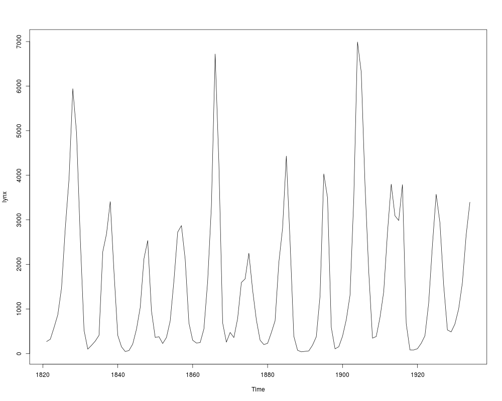
#Figure 1. Plot of lynx time series using plot.ts
plot(lynx)

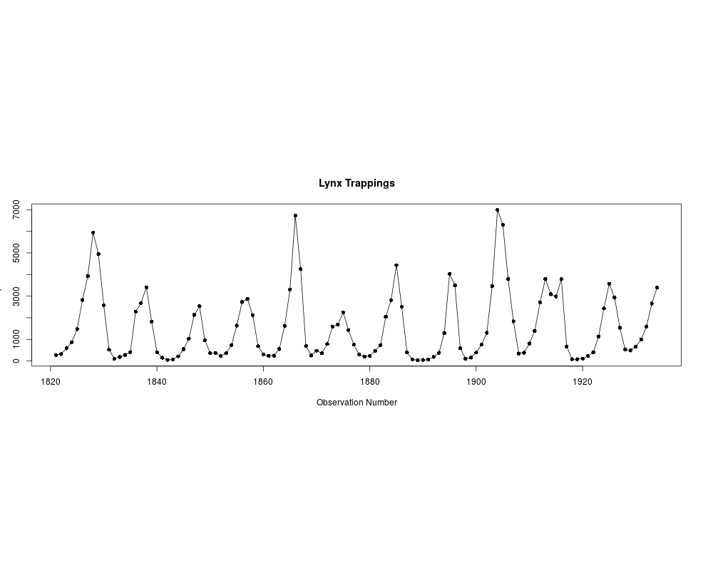
#Figure 2. Plot of lynx series using TimeSeriesPlot
TimeSeriesPlot(lynx, type="o", pch=16, ylab="# pelts", main="Lynx Trappings")

#Figure 3. Trellis plot for Ninemile series
graphics.off() #clear previous graphics
data(Ninemile)
print(TimeSeriesPlot(Ninemile, SubLength=200))

#Figure 4. Partial autocorrelation plot of lynx series 
graphics.off() #clear previous graphics
PacfPlot(log(lynx))

## Not run: #takes some time for all these examples
#Figure 5. Using SelectModel to select the best subset ARz or ARp and
#          comparing BIC and UBIC subset selection.
#
graphics.off() #clear previous graphics
layout(matrix(1:4,ncol=2),respect=TRUE)
ansBICp<-SelectModel(log(lynx),lag.max=15,Criterion="BIC", ARModel="ARp", Best=3)
ansUBICp<-SelectModel(log(lynx),lag.max=15, ARModel="ARp", Best=3)
ansBICz<-SelectModel(log(lynx),lag.max=15,Criterion="BIC", ARModel="ARz", Best=3)
ansUBICz<-SelectModel(log(lynx),lag.max=15, ARModel="ARz", Best=3)
par(mfg=c(1,1))
plot(ansBICp)
par(mfg=c(2,1))
plot(ansUBICp)
par(mfg=c(1,2))
plot(ansBICz)
par(mfg=c(2,2))
plot(ansUBICz)

#Figure 6. Logged spectral density function fitted to square-root of monthly
#          sunspot series using the non-subset AR and subset ARz.
#          AIC and BIC are used for the AR while BIC and UBIC are used
#          for the ARz. Takes about 115 seconds on 3.6 GHz Pentium PC.
graphics.off() #clear previous graphics
layout(matrix(1:4,ncol=2),respect=TRUE)
z<-sqrt(sunspots)
P<-200
pAIC<-SelectModel(z, lag.max=P, ARModel="AR", Best=1, Criterion="AIC")
ARAIC<-FitAR(z, pAIC)
par(mfg=c(1,1))
sdfplot(ARAIC)
title(main="AIC Order Selection")
pBIC<-SelectModel(z, lag.max=P, ARModel="AR", Best=1, Criterion="BIC")
ARBIC<-FitAR(z, pBIC)
par(mfg=c(1,2))
sdfplot(ARBIC)
title(main="BIC Order Selection")
SunspotMonthARzBIC<-SelectModel(z,lag.max=P, ARModel="ARz", Best=1, Criterion="BIC")
ARzBIC<-FitAR(z, SunspotMonthARzBIC)
par(mfg=c(2,1))
sdfplot(ARzBIC)
title(main="BIC Subset Selection")
SunspotMonthARzUBIC<-SelectModel(z,lag.max=P, ARModel="ARz", Best=1)
ARzUBIC<-FitAR(z, SunspotMonthARzUBIC)
par(mfg=c(2,2))
sdfplot(ARzUBIC)
title(main="UBIC Subset Selection")

#Table 3.
#First part of table: AR(1) and AR(2).
#Only timings for GetFitAR and FitAR since the R function ar produces too many
#  warnings and an error message as noted in McLeod and Zhang (2008b, p.12). 
#The ar function with mle option is not recommended.
start.time<-proc.time()
set.seed(661177723)
NREP<-100 #takes about 156 sec
NREP<-10 #takes about 16 sec
ns<-c(50,100,200,500,1000)
ps<-c(1,2) #AR(p), p=1,2
tmsA<-matrix(numeric(4*length(ns)*length(ps)),ncol=4)
ICOUNT<-0
for (IP in 1:length(ps)){
p<-ps[IP]
for (ISIM in 1:length(ns)){
    ICOUNT<-ICOUNT+1
    n<-ns[ISIM]
    ptm <- proc.time()
    for (i in 1:NREP){
        phi<-PacfToAR(runif(p, min=-1, max =1))
        z<-SimulateGaussianAR(phi,n)
        phiHat<-try(GetFitAR(z,p,MeanValue=mean(z))$phiHat)
        }
    t1<-(proc.time() - ptm)[1]
#
    ptm <- proc.time()
    for (i in 1:NREP){
        phi<-PacfToAR(runif(p, min=-1, max =1))
        z<-SimulateGaussianAR(phi,n)
        phiHat<-try(FitAR(z,p,MeanMLEQ=TRUE)$phiHat)
        }
    t2<-(proc.time() - ptm)[1]
#
    ptm <- proc.time()
    for (i in 1:NREP){
        phi<-PacfToAR(runif(p, min=-1, max =1))
        z<-SimulateGaussianAR(phi,n)
        #uncomment this line and next two lines for ar timings -- expect lots of
        #   warnings and an error message!!
        #phiHat<-try(ar(z,aic=FALSE,order.max=p,method="mle")$ar)
        #delete this line and the next one
        phiHat<-NA
    }
    #uncomment this line for ar timings
         #t3<-(proc.time() - ptm)[1]
         t3<-NA #delete this line for ar timings

        tmsA[ICOUNT,]<-c(n,t1,t2,t3)
  } 
} 
rnames<-c(rep("AR(1)", length(ns)),rep("AR(2)", length(ns)) )
cnames<-c("n", "GetFitAR", "FitAR", "ar")  
dimnames(tmsA)<-list(rnames,cnames)
tmsA[,-1]<-round(tmsA[,-1]/NREP,2)
end.time<-proc.time()
total.time<-(end.time-start.time)[1]

#Second part of table: AR(20) and AR(40).
#NOTE: ar is not recommended with method="mle" produces numerous warnings
#      and also takes a long time!
        start.time<-proc.time()
        set.seed(661177723)
        NREP<-100 #takes 7.5 hours
        NREP<-10 #takes 45 minutes
        ns<-c(1000,2000,5000)
        ps<-c(20,40)
        tmsB<-matrix(numeric(4*length(ns)*length(ps)),ncol=4)
        ICOUNT<-0
        for (IP in 1:length(ps)){
        p<-ps[IP]
        phi<-PacfToAR(0.8/(1:p))
        for (ISIM in 1:length(ns)){
            ICOUNT<-ICOUNT+1
            n<-ns[ISIM]
            ptm <- proc.time()
            for (i in 1:NREP){
                z<-SimulateGaussianAR(phi,n)
                phiHat<-try(GetFitAR(z,p,MeanValue=mean(z))$phiHat)
                }
            t1<-(proc.time() - ptm)[1]
            ptm <- proc.time()
            for (i in 1:NREP){
                z<-SimulateGaussianAR(phi,n)
                phiHat<-try(FitAR(z,p,MeanMLEQ=TRUE)$phiHat)
                }
            t2<-(proc.time() - ptm)[1]
            ptm <- proc.time()
            for (i in 1:NREP){
                z<-SimulateGaussianAR(phi,n)
                phiHat<-try(ar(z,aic=FALSE,order.max=p,method="mle")$ar)
                }
            t3<-(proc.time() - ptm)[1]
            tmsB[ICOUNT,]<-c(n,t1,t2,t3)
        } 
        }   
        rnames<-c( rep("AR(20)", length(ns)), rep("AR(40)", length(ns)) )
        cnames<-c("n", "GetFitAR", "FitAR", "ar")  
        dimnames(tmsB)<-list(rnames,cnames)
        tmsB[,-1] <- round(tmsB[,-1]/NREP,2)
        end.time<-proc.time()
        total.time<-(end.time-start.time)[1]

#Figure 7. Comparing Box-Cox analyses using FitAR and MASS
library(MASS)
graphics.off() #clear previous graphics
layout(matrix(c(1,2,1,2),ncol=2))
pvec<-c(1,2,4,10,11)
out<-FitAR(lynx, ARModel="ARp", pvec)
BoxCox(out)
PMAX<-max(pvec)
Xy <- embed(lynx, PMAX + 1)
y <- Xy[, 1]
X <- (Xy[, -1])[, pvec] #pvec != 1
outlm<-lm(y~X)
boxcox(outlm,lambda=seq(0.0,0.6,0.05))

#Figure 8
graphics.off() #clear previous graphics
BoxCox(AirPassengers) #takes about 30 sec

#Figure 9
graphics.off() #clear previous graphics
data(rivers)
BoxCox(rivers)
title(sub="Length of 141 North American Rivers")

#Figure 10
graphics.off() #clear previous graphics
data(USTobacco)
TimeSeriesPlot(USTobacco, aspect=1)

#Figure 11
graphics.off() #clear previous graphics
data(USTobacco)
outUST<-arima(USTobacco, c(0,1,1))
BoxCox(outUST)

#Figure 12. Basic diagnostic plots for ARp fitted to the log lynx series
graphics.off() #clear previous graphics
out<-FitAR(log(lynx), ARModel="ARp", c(1,2,4,10,11))
plot(out, terse=TRUE)

#Figure 13. RSF plot for ARp fitted to log lynx series
graphics.off() #clear previous graphics
out<-FitAR(log(lynx), ARModel="ARp", c(1,2,4,10,11))
rfs(out)

#Table 6. Comparison of bootstrap and large-sample sd
#Use bootstrap to compute standard errors of parameters
#takes about 34 seconds on a 3.6 GHz PC
ptm <- proc.time() #user time
set.seed(2491781) #for reproducibility
R<-100  #number of bootstrap iterations
p<-c(1,2,4,7,10,11)
ans<-FitAR(log(lynx),p)
out<-Boot(ans, R)
fn<-function(z) FitAR(z,p)$zetaHat
sdBoot<-sqrt(diag(var(t(apply(out,fn,MARGIN=2)))))
sdLargeSample<-coef(ans)[,2][1:6]
sd<-matrix(c(sdBoot,sdLargeSample),ncol=2)
dimnames(sd)<-list(names(sdLargeSample),c("Bootstrap","LargeSample"))
ptm<-(proc.time()-ptm)[1]
sd


## End(Not run)

Results

R version 3.3.1 (2016-06-21) -- "Bug in Your Hair"
Copyright (C) 2016 The R Foundation for Statistical Computing
Platform: x86_64-pc-linux-gnu (64-bit)

R is free software and comes with ABSOLUTELY NO WARRANTY.
You are welcome to redistribute it under certain conditions.
Type 'license()' or 'licence()' for distribution details.

R is a collaborative project with many contributors.
Type 'contributors()' for more information and
'citation()' on how to cite R or R packages in publications.

Type 'demo()' for some demos, 'help()' for on-line help, or
'help.start()' for an HTML browser interface to help.
Type 'q()' to quit R.

> library(FitAR)
Loading required package: lattice
Loading required package: leaps
Loading required package: ltsa
Loading required package: bestglm
> png(filename="/home/ddbj/snapshot/RGM3/R_CC/result/FitAR/FitAR-package.Rd_%03d_medium.png", width=480, height=480)
> ### Name: FitAR-package
> ### Title: Fits AR and subset AR models and provides complete model
> ###   building capabilities. FitAR
> ### Aliases: FitAR-package
> ### Keywords: ts package
> 
> ### ** Examples
> 
> #Scripts are given below for all Figures and Tables in McLeod and Zhang (2008b).
> #
> 
> #Figure 1. Plot of lynx time series using plot.ts
> plot(lynx)
> 
> #Figure 2. Plot of lynx series using TimeSeriesPlot
> TimeSeriesPlot(lynx, type="o", pch=16, ylab="# pelts", main="Lynx Trappings")
> 
> #Figure 3. Trellis plot for Ninemile series
> graphics.off() #clear previous graphics
> data(Ninemile)
> print(TimeSeriesPlot(Ninemile, SubLength=200))
> 
> #Figure 4. Partial autocorrelation plot of lynx series 
> graphics.off() #clear previous graphics
> PacfPlot(log(lynx))
> 
> ## Not run: 
> ##D #takes some time for all these examples
> ##D #Figure 5. Using SelectModel to select the best subset ARz or ARp and
> ##D #          comparing BIC and UBIC subset selection.
> ##D #
> ##D graphics.off() #clear previous graphics
> ##D layout(matrix(1:4,ncol=2),respect=TRUE)
> ##D ansBICp<-SelectModel(log(lynx),lag.max=15,Criterion="BIC", ARModel="ARp", Best=3)
> ##D ansUBICp<-SelectModel(log(lynx),lag.max=15, ARModel="ARp", Best=3)
> ##D ansBICz<-SelectModel(log(lynx),lag.max=15,Criterion="BIC", ARModel="ARz", Best=3)
> ##D ansUBICz<-SelectModel(log(lynx),lag.max=15, ARModel="ARz", Best=3)
> ##D par(mfg=c(1,1))
> ##D plot(ansBICp)
> ##D par(mfg=c(2,1))
> ##D plot(ansUBICp)
> ##D par(mfg=c(1,2))
> ##D plot(ansBICz)
> ##D par(mfg=c(2,2))
> ##D plot(ansUBICz)
> ##D 
> ##D #Figure 6. Logged spectral density function fitted to square-root of monthly
> ##D #          sunspot series using the non-subset AR and subset ARz.
> ##D #          AIC and BIC are used for the AR while BIC and UBIC are used
> ##D #          for the ARz. Takes about 115 seconds on 3.6 GHz Pentium PC.
> ##D graphics.off() #clear previous graphics
> ##D layout(matrix(1:4,ncol=2),respect=TRUE)
> ##D z<-sqrt(sunspots)
> ##D P<-200
> ##D pAIC<-SelectModel(z, lag.max=P, ARModel="AR", Best=1, Criterion="AIC")
> ##D ARAIC<-FitAR(z, pAIC)
> ##D par(mfg=c(1,1))
> ##D sdfplot(ARAIC)
> ##D title(main="AIC Order Selection")
> ##D pBIC<-SelectModel(z, lag.max=P, ARModel="AR", Best=1, Criterion="BIC")
> ##D ARBIC<-FitAR(z, pBIC)
> ##D par(mfg=c(1,2))
> ##D sdfplot(ARBIC)
> ##D title(main="BIC Order Selection")
> ##D SunspotMonthARzBIC<-SelectModel(z,lag.max=P, ARModel="ARz", Best=1, Criterion="BIC")
> ##D ARzBIC<-FitAR(z, SunspotMonthARzBIC)
> ##D par(mfg=c(2,1))
> ##D sdfplot(ARzBIC)
> ##D title(main="BIC Subset Selection")
> ##D SunspotMonthARzUBIC<-SelectModel(z,lag.max=P, ARModel="ARz", Best=1)
> ##D ARzUBIC<-FitAR(z, SunspotMonthARzUBIC)
> ##D par(mfg=c(2,2))
> ##D sdfplot(ARzUBIC)
> ##D title(main="UBIC Subset Selection")
> ##D 
> ##D #Table 3.
> ##D #First part of table: AR(1) and AR(2).
> ##D #Only timings for GetFitAR and FitAR since the R function ar produces too many
> ##D #  warnings and an error message as noted in McLeod and Zhang (2008b, p.12). 
> ##D #The ar function with mle option is not recommended.
> ##D start.time<-proc.time()
> ##D set.seed(661177723)
> ##D NREP<-100 #takes about 156 sec
> ##D NREP<-10 #takes about 16 sec
> ##D ns<-c(50,100,200,500,1000)
> ##D ps<-c(1,2) #AR(p), p=1,2
> ##D tmsA<-matrix(numeric(4*length(ns)*length(ps)),ncol=4)
> ##D ICOUNT<-0
> ##D for (IP in 1:length(ps)){
> ##D p<-ps[IP]
> ##D for (ISIM in 1:length(ns)){
> ##D     ICOUNT<-ICOUNT+1
> ##D     n<-ns[ISIM]
> ##D     ptm <- proc.time()
> ##D     for (i in 1:NREP){
> ##D         phi<-PacfToAR(runif(p, min=-1, max =1))
> ##D         z<-SimulateGaussianAR(phi,n)
> ##D         phiHat<-try(GetFitAR(z,p,MeanValue=mean(z))$phiHat)
> ##D         }
> ##D     t1<-(proc.time() - ptm)[1]
> ##D #
> ##D     ptm <- proc.time()
> ##D     for (i in 1:NREP){
> ##D         phi<-PacfToAR(runif(p, min=-1, max =1))
> ##D         z<-SimulateGaussianAR(phi,n)
> ##D         phiHat<-try(FitAR(z,p,MeanMLEQ=TRUE)$phiHat)
> ##D         }
> ##D     t2<-(proc.time() - ptm)[1]
> ##D #
> ##D     ptm <- proc.time()
> ##D     for (i in 1:NREP){
> ##D         phi<-PacfToAR(runif(p, min=-1, max =1))
> ##D         z<-SimulateGaussianAR(phi,n)
> ##D         #uncomment this line and next two lines for ar timings -- expect lots of
> ##D         #   warnings and an error message!!
> ##D         #phiHat<-try(ar(z,aic=FALSE,order.max=p,method="mle")$ar)
> ##D         #delete this line and the next one
> ##D         phiHat<-NA
> ##D     }
> ##D     #uncomment this line for ar timings
> ##D          #t3<-(proc.time() - ptm)[1]
> ##D          t3<-NA #delete this line for ar timings
> ##D 
> ##D         tmsA[ICOUNT,]<-c(n,t1,t2,t3)
> ##D   } 
> ##D } 
> ##D rnames<-c(rep("AR(1)", length(ns)),rep("AR(2)", length(ns)) )
> ##D cnames<-c("n", "GetFitAR", "FitAR", "ar")  
> ##D dimnames(tmsA)<-list(rnames,cnames)
> ##D tmsA[,-1]<-round(tmsA[,-1]/NREP,2)
> ##D end.time<-proc.time()
> ##D total.time<-(end.time-start.time)[1]
> ##D 
> ##D #Second part of table: AR(20) and AR(40).
> ##D #NOTE: ar is not recommended with method="mle" produces numerous warnings
> ##D #      and also takes a long time!
> ##D         start.time<-proc.time()
> ##D         set.seed(661177723)
> ##D         NREP<-100 #takes 7.5 hours
> ##D         NREP<-10 #takes 45 minutes
> ##D         ns<-c(1000,2000,5000)
> ##D         ps<-c(20,40)
> ##D         tmsB<-matrix(numeric(4*length(ns)*length(ps)),ncol=4)
> ##D         ICOUNT<-0
> ##D         for (IP in 1:length(ps)){
> ##D         p<-ps[IP]
> ##D         phi<-PacfToAR(0.8/(1:p))
> ##D         for (ISIM in 1:length(ns)){
> ##D             ICOUNT<-ICOUNT+1
> ##D             n<-ns[ISIM]
> ##D             ptm <- proc.time()
> ##D             for (i in 1:NREP){
> ##D                 z<-SimulateGaussianAR(phi,n)
> ##D                 phiHat<-try(GetFitAR(z,p,MeanValue=mean(z))$phiHat)
> ##D                 }
> ##D             t1<-(proc.time() - ptm)[1]
> ##D             ptm <- proc.time()
> ##D             for (i in 1:NREP){
> ##D                 z<-SimulateGaussianAR(phi,n)
> ##D                 phiHat<-try(FitAR(z,p,MeanMLEQ=TRUE)$phiHat)
> ##D                 }
> ##D             t2<-(proc.time() - ptm)[1]
> ##D             ptm <- proc.time()
> ##D             for (i in 1:NREP){
> ##D                 z<-SimulateGaussianAR(phi,n)
> ##D                 phiHat<-try(ar(z,aic=FALSE,order.max=p,method="mle")$ar)
> ##D                 }
> ##D             t3<-(proc.time() - ptm)[1]
> ##D             tmsB[ICOUNT,]<-c(n,t1,t2,t3)
> ##D         } 
> ##D         }   
> ##D         rnames<-c( rep("AR(20)", length(ns)), rep("AR(40)", length(ns)) )
> ##D         cnames<-c("n", "GetFitAR", "FitAR", "ar")  
> ##D         dimnames(tmsB)<-list(rnames,cnames)
> ##D         tmsB[,-1] <- round(tmsB[,-1]/NREP,2)
> ##D         end.time<-proc.time()
> ##D         total.time<-(end.time-start.time)[1]
> ##D 
> ##D #Figure 7. Comparing Box-Cox analyses using FitAR and MASS
> ##D library(MASS)
> ##D graphics.off() #clear previous graphics
> ##D layout(matrix(c(1,2,1,2),ncol=2))
> ##D pvec<-c(1,2,4,10,11)
> ##D out<-FitAR(lynx, ARModel="ARp", pvec)
> ##D BoxCox(out)
> ##D PMAX<-max(pvec)
> ##D Xy <- embed(lynx, PMAX + 1)
> ##D y <- Xy[, 1]
> ##D X <- (Xy[, -1])[, pvec] #pvec != 1
> ##D outlm<-lm(y~X)
> ##D boxcox(outlm,lambda=seq(0.0,0.6,0.05))
> ##D 
> ##D #Figure 8
> ##D graphics.off() #clear previous graphics
> ##D BoxCox(AirPassengers) #takes about 30 sec
> ##D 
> ##D #Figure 9
> ##D graphics.off() #clear previous graphics
> ##D data(rivers)
> ##D BoxCox(rivers)
> ##D title(sub="Length of 141 North American Rivers")
> ##D 
> ##D #Figure 10
> ##D graphics.off() #clear previous graphics
> ##D data(USTobacco)
> ##D TimeSeriesPlot(USTobacco, aspect=1)
> ##D 
> ##D #Figure 11
> ##D graphics.off() #clear previous graphics
> ##D data(USTobacco)
> ##D outUST<-arima(USTobacco, c(0,1,1))
> ##D BoxCox(outUST)
> ##D 
> ##D #Figure 12. Basic diagnostic plots for ARp fitted to the log lynx series
> ##D graphics.off() #clear previous graphics
> ##D out<-FitAR(log(lynx), ARModel="ARp", c(1,2,4,10,11))
> ##D plot(out, terse=TRUE)
> ##D 
> ##D #Figure 13. RSF plot for ARp fitted to log lynx series
> ##D graphics.off() #clear previous graphics
> ##D out<-FitAR(log(lynx), ARModel="ARp", c(1,2,4,10,11))
> ##D rfs(out)
> ##D 
> ##D #Table 6. Comparison of bootstrap and large-sample sd
> ##D #Use bootstrap to compute standard errors of parameters
> ##D #takes about 34 seconds on a 3.6 GHz PC
> ##D ptm <- proc.time() #user time
> ##D set.seed(2491781) #for reproducibility
> ##D R<-100  #number of bootstrap iterations
> ##D p<-c(1,2,4,7,10,11)
> ##D ans<-FitAR(log(lynx),p)
> ##D out<-Boot(ans, R)
> ##D fn<-function(z) FitAR(z,p)$zetaHat
> ##D sdBoot<-sqrt(diag(var(t(apply(out,fn,MARGIN=2)))))
> ##D sdLargeSample<-coef(ans)[,2][1:6]
> ##D sd<-matrix(c(sdBoot,sdLargeSample),ncol=2)
> ##D dimnames(sd)<-list(names(sdLargeSample),c("Bootstrap","LargeSample"))
> ##D ptm<-(proc.time()-ptm)[1]
> ##D sd
> ##D 
> ## End(Not run)
> 
> 
> 
> 
> 
> 
> 
> dev.off()
null device 
          1 
>