Autoregression Simulation

Description

Simulate a mean-zero stationary Gaussian AR(p) time series.

Usage

SimulateGaussianAR(phi, n = 100, InnovationVariance = 1)

Arguments

Details

The p initial values are simulated using the appropriate multivariate distribution as was suggested in McLeod (1975). The R function rnorm() is used.

Value

A vector of length n, the simulated series

Note

If the process is non-stationary, then random initial values are used determined by the first p innovations.

Author(s)

A.I. McLeod

References

McLeod, A.I. (1975), Derivation of the theoretical autocorrelation function of autoregressive moving-average time series, Applied Statistics 24, 255–256. Percival, D.B. and Walden, A.T. (1993), Spectral Analysis for Physical Applications.

See Also

Boot.FitAR

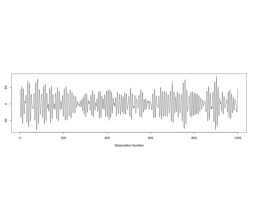
Examples

#Percival and Walden (1993, p.46) illustrated a time series with a 
#very peaked spectrum with the AR(4) with coefficients
#c(2.7607,-3.8106,2.6535,-0.9238) with NID(0,1) innovations.
#
z<-SimulateGaussianAR(c(2.7607,-3.8106,2.6535,-0.9238),1000)
library(lattice)
TimeSeriesPlot(z)

Results

R version 3.3.1 (2016-06-21) -- "Bug in Your Hair"
Copyright (C) 2016 The R Foundation for Statistical Computing
Platform: x86_64-pc-linux-gnu (64-bit)

R is free software and comes with ABSOLUTELY NO WARRANTY.
You are welcome to redistribute it under certain conditions.
Type 'license()' or 'licence()' for distribution details.

R is a collaborative project with many contributors.
Type 'contributors()' for more information and
'citation()' on how to cite R or R packages in publications.

Type 'demo()' for some demos, 'help()' for on-line help, or
'help.start()' for an HTML browser interface to help.
Type 'q()' to quit R.

> library(FitAR)
Loading required package: lattice
Loading required package: leaps
Loading required package: ltsa
Loading required package: bestglm
> png(filename="/home/ddbj/snapshot/RGM3/R_CC/result/FitAR/SimulateGaussianAR.Rd_%03d_medium.png", width=480, height=480)
> ### Name: SimulateGaussianAR
> ### Title: Autoregression Simulation
> ### Aliases: SimulateGaussianAR
> ### Keywords: ts
> 
> ### ** Examples
> 
> #Percival and Walden (1993, p.46) illustrated a time series with a 
> #very peaked spectrum with the AR(4) with coefficients
> #c(2.7607,-3.8106,2.6535,-0.9238) with NID(0,1) innovations.
> #
> z<-SimulateGaussianAR(c(2.7607,-3.8106,2.6535,-0.9238),1000)
> library(lattice)
> TimeSeriesPlot(z)
> 
> 
> 
> 
> 
> dev.off()
null device 
          1 
>