R Graphical Manual

Browse All

Last data update: 2014.03.03

R: Multi-Panel or Single-Panel Time Series Plot with...

TimeSeriesPlot

R Documentation

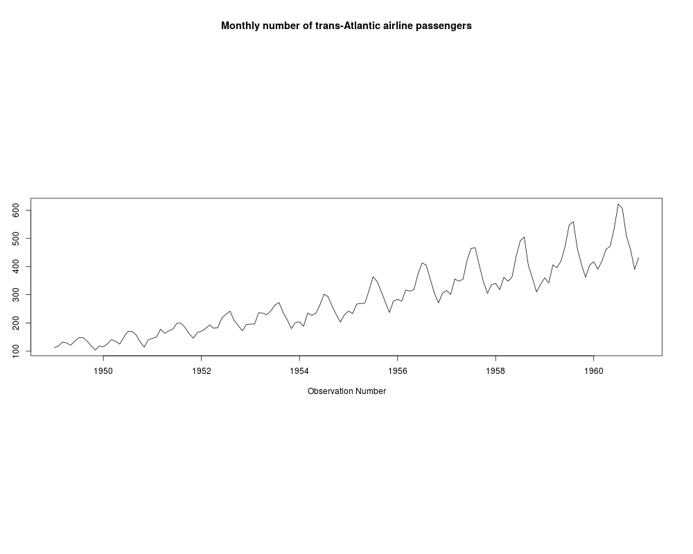
Multi-Panel or Single-Panel Time Series Plot with Aspect-Ratio Control

Description

Cleveland (1993) pointed out that the aspect-ratio is important in graphically showing the rate-of-change or shape information. For many time series, it is preferably to set this ratio to 0.25 than the default. In general, Cleveland (1993) shows that the best choice of aspect-ratio is often obtained by if the average apparent absolute slope in the graph is about 45 deg. But for many stationary time series, this would result in an aspect-ratio which would be too small. As a comprise we have chosen a default of 0.25 but the user can select other choices.

Usage

TimeSeriesPlot(z, SubLength = Inf, aspect = 0.25, type="l", xlab = "Observation Number",
   ylab=NULL, main=NULL, ...)

Arguments

`z`	ts object or vector, time series data
`SubLength`	maximum number of data points per panel. Default SubLength=Inf and regular graphics. For trellis graphics, set SubLength to a finite value.
`aspect`	optional setting for the aspect-ratio
`type`	plot type, default type="l" join points with lines
`xlab`	label for horizontal axis
`ylab`	optional label for vertical axis
`main`	optional title
`...`	optional arguments passed to `xyplot`

Details

If z has attribute "title" containing a character string, this is used on the plot. Time series input using the function Readts always have this attribute set.

Value

If SubLength is finite, the lattice package is used and a graphic object of class trellis is produced. Otherwise, the standard R graphics system is used and the plot is produced as a side-effect and there is no output.

Note

Requires lattice library

Author(s)

A.I. McLeod

References

W.S. Cleveland (1993), Visualizing Data.

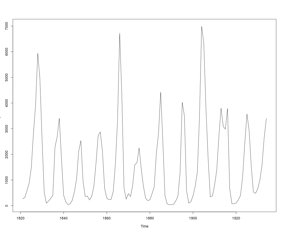
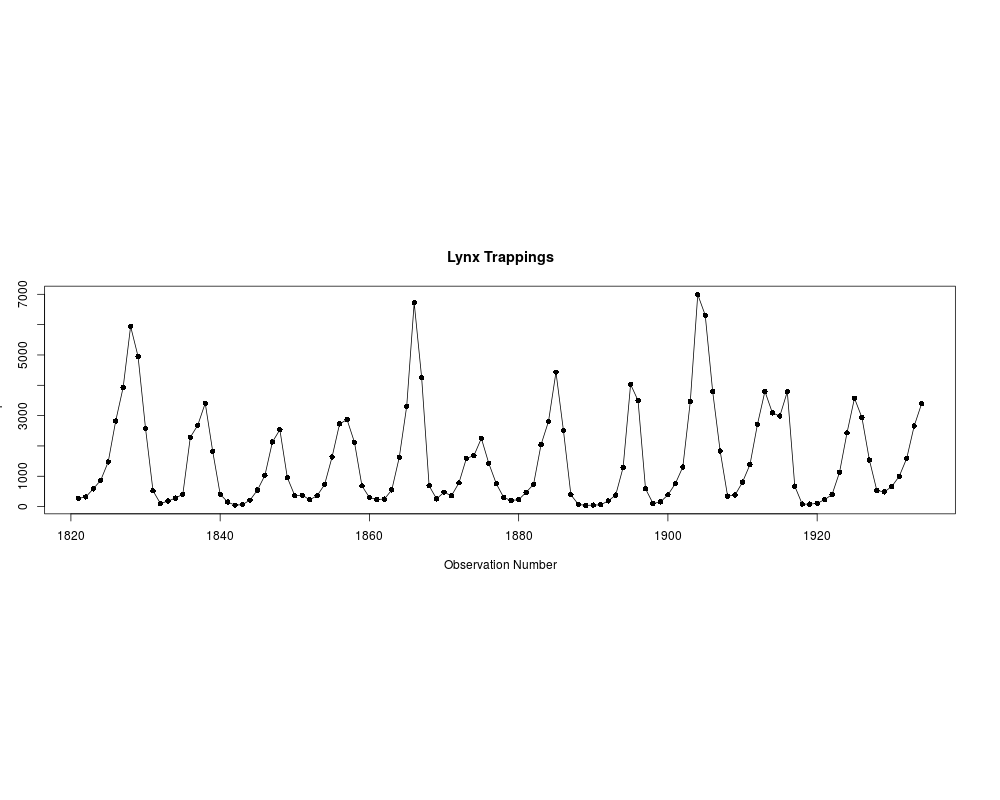
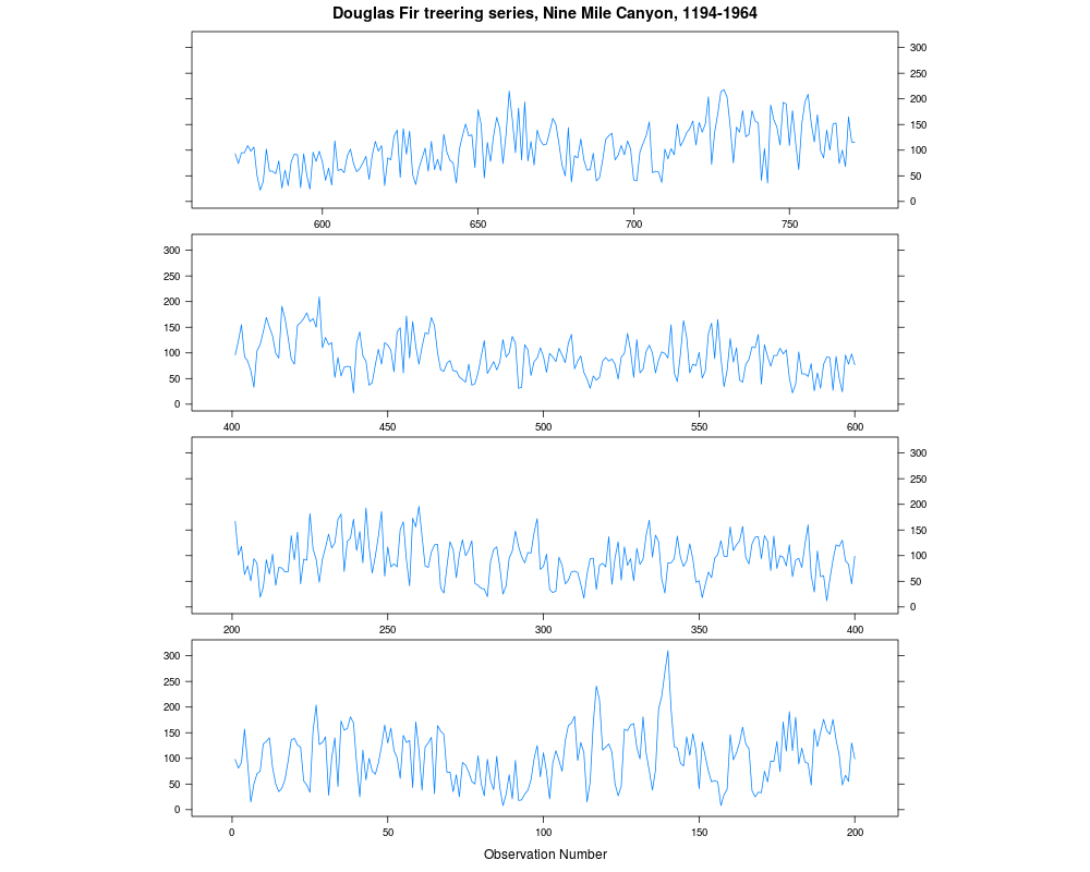
Examples

#from built-in datasets
 TimeSeriesPlot(AirPassengers)
 title(main="Monthly number of trans-Atlantic airline passengers")
#
#compare plots for lynx series
plot(lynx)
TimeSeriesPlot(lynx, type="o", pch=16, ylab="# pelts", main="Lynx Trappings")
#
#lattice style plot
data(Ninemile)
TimeSeriesPlot(Ninemile, SubLength=200)

Results


R version 3.3.1 (2016-06-21) -- "Bug in Your Hair"
Copyright (C) 2016 The R Foundation for Statistical Computing
Platform: x86_64-pc-linux-gnu (64-bit)

R is free software and comes with ABSOLUTELY NO WARRANTY.
You are welcome to redistribute it under certain conditions.
Type 'license()' or 'licence()' for distribution details.

R is a collaborative project with many contributors.
Type 'contributors()' for more information and
'citation()' on how to cite R or R packages in publications.

Type 'demo()' for some demos, 'help()' for on-line help, or
'help.start()' for an HTML browser interface to help.
Type 'q()' to quit R.

> library(FitAR)
Loading required package: lattice
Loading required package: leaps
Loading required package: ltsa
Loading required package: bestglm
> png(filename="/home/ddbj/snapshot/RGM3/R_CC/result/FitAR/TimeSeriesPlot.Rd_%03d_medium.png", width=480, height=480)
> ### Name: TimeSeriesPlot
> ### Title: Multi-Panel or Single-Panel Time Series Plot with Aspect-Ratio
> ###   Control
> ### Aliases: TimeSeriesPlot
> ### Keywords: ts
> 
> ### ** Examples
> 
> #from built-in datasets
>  TimeSeriesPlot(AirPassengers)
>  title(main="Monthly number of trans-Atlantic airline passengers")
> #
> #compare plots for lynx series
> plot(lynx)
> TimeSeriesPlot(lynx, type="o", pch=16, ylab="# pelts", main="Lynx Trappings")
> #
> #lattice style plot
> data(Ninemile)
> TimeSeriesPlot(Ninemile, SubLength=200)
> 
> 
> 
> 
> 
> dev.off()
null device 
          1 
>