R Graphical Manual

Browse All

Last data update: 2014.03.03

R: Genetic Algorithms

ga	R Documentation

Genetic Algorithms

Description

Maximization of a fitness function using genetic algorithms (GAs). Local search using general-purpose optimisation algorithms can be applied stochastically to exploit interesting regions. The algorithm can be run sequentially or in parallel using an explicit master-slave parallelisation.

Usage

ga(type = c("binary", "real-valued", "permutation"), 
   fitness, ...,
   min, max, nBits,
   population = gaControl(type)$population,
   selection = gaControl(type)$selection,
   crossover = gaControl(type)$crossover, 
   mutation = gaControl(type)$mutation,
   popSize = 50, 
   pcrossover = 0.8, 
   pmutation = 0.1, 
   elitism = base::max(1, round(popSize*0.05)), 
   updatePop = FALSE,
   postFitness = NULL,
   maxiter = 100,
   run = maxiter,
   maxFitness = Inf,
   names = NULL,
   suggestions = NULL, 
   optim = FALSE,
   optimArgs = list(method = "L-BFGS-B", 
                    poptim = 0.05,
                    pressel = 0.5,
                    control = list(fnscale = -1, maxit = 100)),
   keepBest = FALSE,
   parallel = FALSE,
   monitor = if(interactive()) 
               { if(is.RStudio()) gaMonitor else gaMonitor2 } 
             else FALSE,
   seed = NULL)

Arguments

type

the type of genetic algorithm to be run depending on the nature of decision variables. Possible values are:

`"binary"`	for binary representations of decision variables.
`"real-valued"`	for optimization problems where the decision variables are floating-point representations of real numbers.
`"permutation"`	for problems that involves reordering of a list.

fitness

the fitness function, any allowable R function which takes as input an individual string representing a potential solution, and returns a numerical value describing its “fitness”.

...

additional arguments to be passed to the fitness function. This allows to write fitness functions that keep some variables fixed during the search.

min

a vector of length equal to the decision variables providing the minimum of the search space in case of real-valued or permutation encoded optimizations.

max

a vector of length equal to the decision variables providing the maximum of the search space in case of real-valued or permutation encoded optimizations.

nBits

a value specifying the number of bits to be used in binary encoded optimizations.

population

an R function for randomly generating an initial population. See ga_Population for available functions.

selection

an R function performing selection, i.e. a function which generates a new population of individuals from the current population probabilistically according to individual fitness. See ga_Selection for available functions.

crossover

an R function performing crossover, i.e. a function which forms offsprings by combining part of the genetic information from their parents. See ga_Crossover for available functions.

mutation

an R function performing mutation, i.e. a function which randomly alters the values of some genes in a parent chromosome. See ga_Mutation for available functions.

popSize

the population size.

updatePop

a logical defaulting to FALSE. If set at TRUE the first attribute attached to the value returned by the user-defined fitness function is used to update the population.
Be careful though, this is an experimental feature!

postFitness

a user-defined function which, if provided, receives the current ga-class object as input, performs post fitness-evaluation steps, then returns an updated version of the object which is used to update the GA search.
Be careful though, this is an experimental feature!

pcrossover

the probability of crossover between pairs of chromosomes. Typically this is a large value and by default is set to 0.8.

pmutation

the probability of mutation in a parent chromosome. Usually mutation occurs with a small probability, and by default is set to 0.1.

elitism

the number of best fitness individuals to survive at each generation. By default the top 5% individuals will survive at each iteration.

maxiter

the maximum number of iterations to run before the GA search is halted.

run

the number of consecutive generations without any improvement in the best fitness value before the GA is stopped.

maxFitness

the upper bound on the fitness function after that the GA search is interrupted.

names

a vector of character strings providing the names of decision variables.

suggestions

a matrix of solutions strings to be included in the initial population. If provided the number of columns must match the number of decision variables.

optim

a logical defaulting to FALSE determining whether or not a local search using general-purpose optimisation algorithms should be used. See argument optimArgs for further details and finer control.

optimArgs

a list controlling the local search algorithm with the following components:

method: a string specifying the general-purpose optimisation method to be used, by default is set to "L-BFGS-B". Other possible methods are those reported in optim.
poptim: a value in the range [0,1] specifying the probability of performing a local search at each iteration of GA (default 0.1).
pressel: a value in the range [0,1] specifying the pressure selection (default 0.5). The local search is started from a random solution selected with probability proportional to fitness. High values of pressel tend to select the solutions with the largest fitness, whereas low values of pressel assign quasi-uniform probabilities to any solution.
control: a list of control parameters. See 'Details' section in optim.

keepBest

a logical argument specifying if best solutions at each iteration should be saved in a slot called bestSol. See ga-class.

parallel

a logical argument specifying if parallel computing should be used (TRUE) or not (FALSE, default) for evaluating the fitness function. This argument could also be used to specify the number of cores to employ; by default, this is taken from detectCores. Finally, the functionality of parallelization depends on system OS: on Windows only 'snow' type functionality is available, while on Unix/Linux/Mac OSX both 'snow' and 'multicore' (default) functionalities are available.

monitor

a logical or an R function which takes as input the current state of the ga-class object and show the evolution of the search. By default, for interactive sessions, the function gaMonitor or gaMonitor2, depending on whether or not is an RStudio session, prints the average and best fitness values at each iteration. If set to plot these information are plotted on a graphical device. Other functions can be written by the user and supplied as argument. In non interactive sessions, by default monitor = FALSE so any output is suppressed.

seed

an integer value containing the random number generator state. This argument can be used to replicate the results of a GA search. Note that if parallel computing is required, the doRNG package must be installed.

Details

Genetic algorithms (GAs) are stochastic search algorithms inspired by the basic principles of biological evolution and natural selection. GAs simulate the evolution of living organisms, where the fittest individuals dominate over the weaker ones, by mimicking the biological mechanisms of evolution, such as selection, crossover and mutation.

The GA package is a collection of general purpose functions that provide a flexible set of tools for applying a wide range of genetic algorithm methods.

The ga function enables the application of GAs to problems where the decision variables are encoded as "binary", "real-valued", or "permutation" strings.

Default genetic operators are set via gaControl. To retrieve the currently set operators:

gaControl("binary")

gaControl("real-valued")

gaControl("permutation")

Value

Returns an object of class ga-class. See ga-class for a description of available slots information.

Author(s)

Luca Scrucca luca.scrucca@unipg.it

References

Back T., Fogel D., Michalewicz Z. (2000). Evolutionary Computation 1: Basic Algorithms and Operators. IOP Publishing Ltd., Bristol and Philadelphia.

Back T., Fogel D., Michalewicz Z. (2000b). Evolutionary Computation 2: Advanced Algorithms and Operators. IOP Publishing Ltd., Bristol and Philadelphia.

Coley D. (1999). An Introduction to Genetic Algorithms for Scientists and Engineers. World Scientific Pub. Co. Inc., Singapore.

Eiben A., Smith J. (2003). Introduction to Evolutionary Computing. Springer-Verlag, Berlin Heidelberg.

Goldberg D. (1989). Genetic Algorithms in Search, Optimization, and Machine Learning. Addison-Wesley Professional, Boston, MA.

Haupt R. L., Haupt S. E. (2004). Practical Genetic Algorithms. 2nd edition. John Wiley & Sons, New York.

Luke S. (2013) Essentials of Metaheuristics, 2nd edition. Lulu. Freely available at http://cs.gmu.edu/~sean/book/metaheuristics/.

Scrucca L. (2013). GA: A Package for Genetic Algorithms in R. Journal of Statistical Software, 53(4), 1-37, http://www.jstatsoft.org/v53/i04/.

Scrucca L. (2016). On some extensions to GA package: hybrid optimisation, parallelisation and islands evolution. Submitted to R Journal. Pre-print available at http://arxiv.org/abs/1605.01931.

Simon D. (2013) Evolutionary Optimization Algorithms. John Wiley & Sons.

Sivanandam S., Deepa S. (2007). Introduction to Genetic Algorithms. Springer-Verlag, Berlin Heidelberg.

Yu X., Gen M. (2010). Introduction to Evolutionary Algorithms. Springer-Verlag, Berlin Heidelberg.

Examples

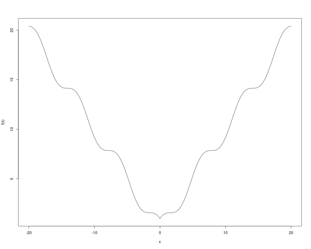
# 1) one-dimensional function
f <- function(x)  abs(x)+cos(x)
curve(f, -20, 20)

fitness <- function(x) -f(x)
GA <- ga(type = "real-valued", fitness = fitness, min = -20, max = 20)
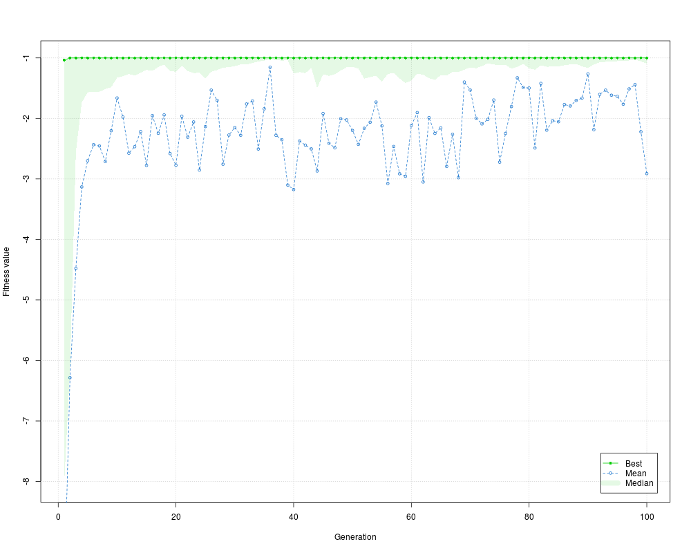
summary(GA)
plot(GA)

curve(f, -20, 20)
abline(v = GA@solution, lty = 3)

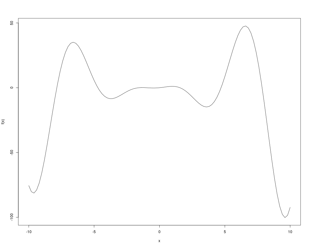
# 2) one-dimensional function
f <- function(x)  (x^2+x)*cos(x) # -10 < x < 10
curve(f, -10, 10)

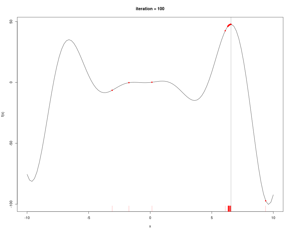
# write your own tracing function
monitor <- function(obj) 
{ 
  curve(f, -10, 10, main = paste("iteration =", obj@iter))
  points(obj@population, obj@fitness, pch = 20, col = 2)
  rug(obj@population, col = 2)
  Sys.sleep(0.2)
}
## Not run: 
GA <- ga(type = "real-valued", fitness = f, min = -10, max = 10, monitor = monitor)

## End(Not run)
# or if you want to suppress the tracing
GA <- ga(type = "real-valued", fitness = f, min = -10, max = 10, monitor = NULL)
summary(GA)

monitor(GA)
abline(v = GA@solution, lty = 3)

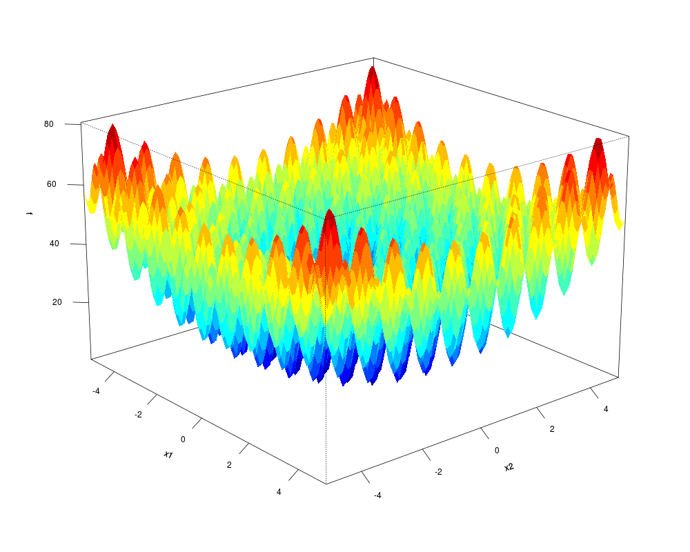
# 3) two-dimensional Rastrigin function

Rastrigin <- function(x1, x2)
{
  20 + x1^2 + x2^2 - 10*(cos(2*pi*x1) + cos(2*pi*x2))
}

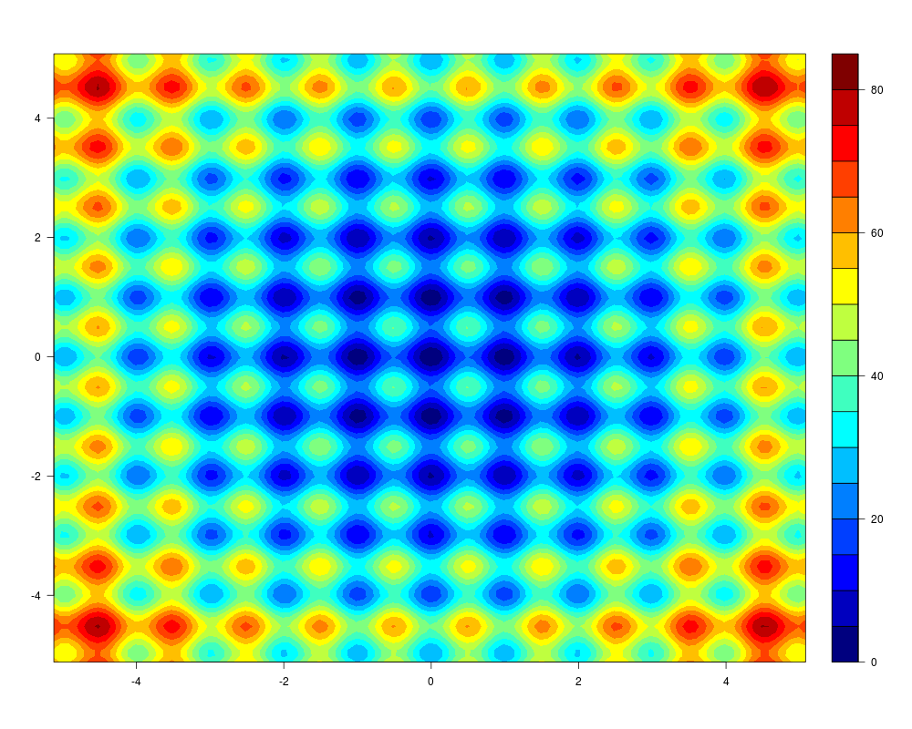
x1 <- x2 <- seq(-5.12, 5.12, by = 0.1)
f <- outer(x1, x2, Rastrigin)
persp3D(x1, x2, f, theta = 50, phi = 20)
filled.contour(x1, x2, f, color.palette = jet.colors)

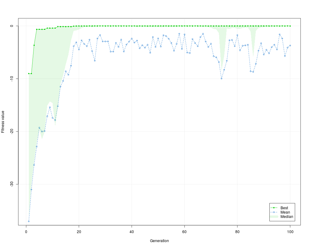
GA <- ga(type = "real-valued", fitness =  function(x) -Rastrigin(x[1], x[2]),
         min = c(-5.12, -5.12), max = c(5.12, 5.12), 
         popSize = 50, maxiter = 100)
summary(GA)
plot(GA)

# 4) Parallel GA
# Simple example of an expensive fitness function obtained artificially by
# introducing a pause statement. 
## Not run: 
Rastrigin <- function(x1, x2)
{
  Sys.sleep(0.1)
  20 + x1^2 + x2^2 - 10*(cos(2*pi*x1) + cos(2*pi*x2))
}

system.time(GA1 <- ga(type = "real-valued", 
                      fitness =  function(x) -Rastrigin(x[1], x[2]),
                      min = c(-5.12, -5.12), max = c(5.12, 5.12), 
                      popSize = 50, maxiter = 100, monitor = FALSE,
                      seed = 12345))

system.time(GA2 <- ga(type = "real-valued", 
                      fitness =  function(x) -Rastrigin(x[1], x[2]),
                      min = c(-5.12, -5.12), max = c(5.12, 5.12), 
                      popSize = 50, maxiter = 100, monitor = FALSE,
                      seed = 12345, parallel = TRUE))

## End(Not run)

# 5) Hybrid GA
# Example of GA with local search 

Rastrigin <- function(x1, x2)
{
  20 + x1^2 + x2^2 - 10*(cos(2*pi*x1) + cos(2*pi*x2))
}

GA <- ga(type = "real-valued", 
         fitness =  function(x) -Rastrigin(x[1], x[2]),
         min = c(-5.12, -5.12), max = c(5.12, 5.12), 
         popSize = 50, maxiter = 100,
         optim = TRUE)
summary(GA)

Results


R version 3.3.1 (2016-06-21) -- "Bug in Your Hair"
Copyright (C) 2016 The R Foundation for Statistical Computing
Platform: x86_64-pc-linux-gnu (64-bit)

R is free software and comes with ABSOLUTELY NO WARRANTY.
You are welcome to redistribute it under certain conditions.
Type 'license()' or 'licence()' for distribution details.

R is a collaborative project with many contributors.
Type 'contributors()' for more information and
'citation()' on how to cite R or R packages in publications.

Type 'demo()' for some demos, 'help()' for on-line help, or
'help.start()' for an HTML browser interface to help.
Type 'q()' to quit R.

> library(GA)
Loading required package: foreach
Loading required package: iterators
Package 'GA' version 3.0.2
Type 'citation("GA")' for citing this R package in publications.
> png(filename="/home/ddbj/snapshot/RGM3/R_CC/result/GA/ga.Rd_%03d_medium.png", width=480, height=480)
> ### Name: ga
> ### Title: Genetic Algorithms
> ### Aliases: ga show,ga-method print,ga-method
> ### Keywords: optimize
> 
> ### ** Examples
> 
> # 1) one-dimensional function
> f <- function(x)  abs(x)+cos(x)
> curve(f, -20, 20)
> 
> fitness <- function(x) -f(x)
> GA <- ga(type = "real-valued", fitness = fitness, min = -20, max = 20)
> summary(GA)
+-----------------------------------+
|         Genetic Algorithm         |
+-----------------------------------+

GA settings: 
Type                  =  real-valued 
Population size       =  50 
Number of generations =  100 
Elitism               =  2 
Crossover probability =  0.8 
Mutation probability  =  0.1 
Search domain = 
     x1
Min -20
Max  20

GA results: 
Iterations             = 100 
Fitness function value = -1.000032 
Solution = 
                x1
[1,] -3.230359e-05
> plot(GA)
> 
> curve(f, -20, 20)
> abline(v = GA@solution, lty = 3)
> 
> # 2) one-dimensional function
> f <- function(x)  (x^2+x)*cos(x) # -10 < x < 10
> curve(f, -10, 10)
> 
> # write your own tracing function
> monitor <- function(obj) 
+ { 
+   curve(f, -10, 10, main = paste("iteration =", obj@iter))
+   points(obj@population, obj@fitness, pch = 20, col = 2)
+   rug(obj@population, col = 2)
+   Sys.sleep(0.2)
+ }
> ## Not run: 
> ##D GA <- ga(type = "real-valued", fitness = f, min = -10, max = 10, monitor = monitor)
> ## End(Not run)
> # or if you want to suppress the tracing
> GA <- ga(type = "real-valued", fitness = f, min = -10, max = 10, monitor = NULL)
> summary(GA)
+-----------------------------------+
|         Genetic Algorithm         |
+-----------------------------------+

GA settings: 
Type                  =  real-valued 
Population size       =  50 
Number of generations =  100 
Elitism               =  2 
Crossover probability =  0.8 
Mutation probability  =  0.1 
Search domain = 
     x1
Min -10
Max  10

GA results: 
Iterations             = 100 
Fitness function value = 47.70562 
Solution = 
           x1
[1,] 6.560737
> 
> monitor(GA)
> abline(v = GA@solution, lty = 3)
> 
> # 3) two-dimensional Rastrigin function
> 
> Rastrigin <- function(x1, x2)
+ {
+   20 + x1^2 + x2^2 - 10*(cos(2*pi*x1) + cos(2*pi*x2))
+ }
> 
> x1 <- x2 <- seq(-5.12, 5.12, by = 0.1)
> f <- outer(x1, x2, Rastrigin)
> persp3D(x1, x2, f, theta = 50, phi = 20)
> filled.contour(x1, x2, f, color.palette = jet.colors)
> 
> GA <- ga(type = "real-valued", fitness =  function(x) -Rastrigin(x[1], x[2]),
+          min = c(-5.12, -5.12), max = c(5.12, 5.12), 
+          popSize = 50, maxiter = 100)
> summary(GA)
+-----------------------------------+
|         Genetic Algorithm         |
+-----------------------------------+

GA settings: 
Type                  =  real-valued 
Population size       =  50 
Number of generations =  100 
Elitism               =  2 
Crossover probability =  0.8 
Mutation probability  =  0.1 
Search domain = 
       x1    x2
Min -5.12 -5.12
Max  5.12  5.12

GA results: 
Iterations             = 100 
Fitness function value = -1.470001e-05 
Solution = 
                x1           x2
[1,] -0.0001618461 0.0002188643
> plot(GA)
> 
> # 4) Parallel GA
> # Simple example of an expensive fitness function obtained artificially by
> # introducing a pause statement. 
> ## Not run: 
> ##D Rastrigin <- function(x1, x2)
> ##D {
> ##D   Sys.sleep(0.1)
> ##D   20 + x1^2 + x2^2 - 10*(cos(2*pi*x1) + cos(2*pi*x2))
> ##D }
> ##D 
> ##D system.time(GA1 <- ga(type = "real-valued", 
> ##D                       fitness =  function(x) -Rastrigin(x[1], x[2]),
> ##D                       min = c(-5.12, -5.12), max = c(5.12, 5.12), 
> ##D                       popSize = 50, maxiter = 100, monitor = FALSE,
> ##D                       seed = 12345))
> ##D 
> ##D system.time(GA2 <- ga(type = "real-valued", 
> ##D                       fitness =  function(x) -Rastrigin(x[1], x[2]),
> ##D                       min = c(-5.12, -5.12), max = c(5.12, 5.12), 
> ##D                       popSize = 50, maxiter = 100, monitor = FALSE,
> ##D                       seed = 12345, parallel = TRUE))
> ## End(Not run)
> 
> # 5) Hybrid GA
> # Example of GA with local search 
> 
> Rastrigin <- function(x1, x2)
+ {
+   20 + x1^2 + x2^2 - 10*(cos(2*pi*x1) + cos(2*pi*x2))
+ }
> 
> GA <- ga(type = "real-valued", 
+          fitness =  function(x) -Rastrigin(x[1], x[2]),
+          min = c(-5.12, -5.12), max = c(5.12, 5.12), 
+          popSize = 50, maxiter = 100,
+          optim = TRUE)
> summary(GA)
+-----------------------------------+
|         Genetic Algorithm         |
+-----------------------------------+

GA settings: 
Type                  =  real-valued 
Population size       =  50 
Number of generations =  100 
Elitism               =  2 
Crossover probability =  0.8 
Mutation probability  =  0.1 
Search domain = 
       x1    x2
Min -5.12 -5.12
Max  5.12  5.12

GA results: 
Iterations             = 100 
Fitness function value = 0 
Solution = 
     x1 x2
[1,]  0  0
> 
> 
> 
> 
> 
> 
> dev.off()
null device 
          1 
>